Animal Ecology

Spatio-temporal Changes in Wildlife Habitat Quality in the Middle and Lower Reaches of the Yangtze River from 1980 to 2100 based on the InVEST Model

  • LI Qing , 1 ,
  • ZHOU Yong , 1, * ,
  • Mary Ann CUNNINGHAM 2 ,
  • XU Tao 1
Expand
  • 1. The College of Urban & Environmental Sciences, Central China Normal University, Wuhan 430079, China
  • 2. Department of Earth Science and Geography, Vassar College, Poughkeepsie, New York 12603, USA
*ZHOU Yong, E-mail:

LI Qing, E-mail:

Received date: 2020-07-31

  Accepted date: 2020-09-20

  Online published: 2021-03-30

Supported by

National Natural Science Foundation of China(41271534)

China Scholarship Council(201906770044)

Abstract

The Yangtze River (YZR) regions have experienced rapid changes after opening up to economic reforms, and human activities have changed the land cover, ecology, and wildlife habitat quality. However, the specific ways in which those influencing factors changed the habitat quality during different periods remain unknown. This study assessed the wildlife habitat quality of the middle and lower YZR in the past (1980-2018) and in future scenarios (2050, 2100). We analyzed the relationships between habitat quality and various topological social-economic factors, and then mapped and evaluated the changes in habitat quality by using the Integrated Valuation of Environmental Services and Tradeoffs (InVEST) model. The results show that the slope (R = 0.502, P < 0.01, in 2015), elevation (R = 0.003, P < 0.05, in 2015), population density (R = -0.299, P < 0.01, in 2015), and NDVI (R = 0.366, P < 0.01, in 2015) in the study area were significantly correlated with habitat quality from 2000 to 2015. During the period of 1980-2018, 61.93% of the study area experienced habitat degradation and 38.07% of the study area had improved habitat quality. In the future, the habitat quality of the study area will decline under either the A2 scenario (high level of population density, low environmental technology input, and high traditional energy cost) or the B2 scenario (medium level of population density, medium green technology and lack of cooperation of regional governments). The results also showed that habitat in the lower reaches or north of the YZR had degraded more than in the middle reaches or the south of YZR. Therefore, regional development should put more effort into environmental protection, curb population growth, and encourage green technology innovation. Inter-province cooperation is necessary when dealing with ecological problems. This study can serve as a scientific reference for regional wildlife protection and similar investigations in different areas.

Cite this article

LI Qing , ZHOU Yong , Mary Ann CUNNINGHAM , XU Tao . Spatio-temporal Changes in Wildlife Habitat Quality in the Middle and Lower Reaches of the Yangtze River from 1980 to 2100 based on the InVEST Model[J]. Journal of Resources and Ecology, 2021 , 12(1) : 43 -55 . DOI: 10.5814/j.issn.1674-764x.2021.01.005

1 Introduction

Habitat quality is the ability of the land to provide essential habitat components for a particular species, and it determines the wildlife population status in the landscape (Johnson, 2007). Changes in land use affect habitat quality, which often has an impact on the reproduction and survival of wildlife through variations in available natural resources (Dai et al., 2019, Whittington et al., 2019). Humans have extensively altered the global environment (Nadakavukaren and Caravanos, 2020), changed global biogeochemical cycles (Abbott et al., 2019), transformed land, and changed the habitat quality for wildlife (Powers and Jetz, 2019); all of which have adversely affected ecosystem functions and services. Places where habitat degradation is interlinked with the loss of biodiversity (Amato et al., 2013; Manangkalangi et al., 2019) and environmental degradation have difficulty in achieving sustainable development (Pulliam, 2000).
Researchers worldwide have put tremendous effort into assessing habitat quality in order to provide scientific information on the drivers and changes of habitat so that they may improve the local ecosystem (Van Horne, 1983; Whittington et al., 2019). Earlier studies started with field surveys of biodiversity and habitat which focused on a particular species at a local level, such as deer (Pettorelli et al., 2001), fish (Manangkalangi et al., 2019), butterflies (Öckinger et al., 2009), or tigers (Smith et al., 1998). These studies created a knowledge basis for assessing the habitat quality for certain species in similar areas. Nevertheless, studies based on field trips are costly, and so few of these studies tracked the species over many years. Therefore, they are not helpful when the policy-makers want to develop a natural protection plan at a large scale, which requires consideration of multiple species.
The developments in geographic science and remote sensing science allow habitat quality assessments at a large scale. Habitat quality assessment methods based on suitable ecological indicators for certain species have been developed (Niemi and McDonald, 2004; Erdozain et al., 2019; Rao et al., 2019). One strategy combines remote sensing-based indicators with field data to assess the potentially suitable habitat for a certain species. Another type of research method evaluates habitat quality via ecological simulation models.
The Natural and Capital Project of Stanford University has developed the Integrated Valuation of Ecosystem Services and Trade-offs (InVEST) model, which produces habitat quality maps from limited data on biodiversity (Nelson et al., 2009), and has proven to be a powerful tool for monitoring the variation in habitat quality for wildlife. Scholars worldwide have analyzed the impacts of land use and land cover changes on habitat quality by using this model in systems with different social and economic backgrounds.
There are three basic types of research on this topic. Most of the studies have focused on a small area, such as a mountain (Zhou and Zhang, 2011), a river (Li et al., 2019), or a city (Zhu et al., 2020). The first type includes studies on the impact of specific land use change projects on habitat quality, such as Zhou et al. (2010) who explored different types of forest ecosystem effects on soil conservation in the mountain areas of Beijing based on InVEST Model. Zhong and Wang (2017) evaluated the effect of land consolidation in Da’an City on habitat quality based on the InVEST model. Hack et al. (2020) assessed the individual and combined impacts of built-up areas, first- and second-order roads, water pollution from urban drainage, and wastewater discharge on habitat quality within a 200 m wide river corridor in the Pochote River in Leoacuten. The second type includes studies on the impact of land use change on habitat quality combined with land use prediction models. For example, Jiang et al. (2017) modeled the potential impacts of urban ecosystem changes on carbon storage under different scenarios by linking the CLUE-S and InVEST models. Upadhaya and Dwivedi (2019) assessed the dynamic effects of land use changes on habitat quality (2010-2017) in the Alabaha River watershed. They used Markov Multi-Layer Perceptron to predict LUCs in 2022 and 2030, and used FRAGSTATS to assess changes in landscape configuration and composition over time. Chu et al. (2018) investigated the landscape pattern and habitat quality based on the CA-Markov and InVEST Model in the Hubei section of the Three Gorges Reservoir Area. The third type of studies examines the relationships between habitat quality and local natural and socio-economic factors. For example, Berta et al. (2020) analyzed the habitat quality variations from 1988 to 2018 in Winike watershed and assessed the relationships between population density, land use intensity, elevation, and slope.
Few studies have quantified the interrelationships between human activities and habitat quality at a large scale in China. After the Chinese economic reform, an increasing amount of construction land replaced cropland, resulting in the loss and fragmentation of habitats (Liu et al., 2003). China has enacted and implemented a series of principles, policies, laws, and measures for environmental protection since the 1980s (Liang and Yang, 2019). So how do the economic factors or natural factors impact habitat quality in different provinces? In this study, we take seven provinces of the middle and lower reaches of the Yangtze River (YZR) as the study area, and compare the spatio-temporal changes of habitat quality among the provinces. YZR is the home of diverse wildlife, including 378 species of fish, more than 280 species of mammals, 145 species of amphibians, and 166 species of reptiles, although the area is threatened by declining in habitat quality and biodiversity loss (Barter et al., 2006). The economic development in this area is also vital to China. Based on a previous study of land use and land cover (LULC) changes in the future (Liu et al., 2017) and available quantitative economic and natural data, the aims of this study are as follows: 1) reveal the spatial-temporal variations of land use and land cover changes in the middle and lower reaches of the Yangtze River in the past (1980-2018) and in the future (2050; 2100); 2) assess the habitat quality changes of this region from 1980 to 2100; and 3) explore the spatio-temporal pattern of habitat quality and its influencing factors in the middle and lower reaches of YZR.

2 Materials and methods

2.1 Study area

The middle and lower YZR crosses 7 provinces in China, including Hubei Province, Hunan Province, Jiangxi Province, Anhui Province, Jiangsu Province, Zhejiang Province, and Shanghai City. The average annual temperature in this area varies from 14 ℃ to 18 ℃ and annual precipitation spans 1000 mm to 1500 mm. This region is a substantial production base for grains, vegetable oil, and cotton in China, and it is the most water-rich region in China. Famous freshwater lakes in the region include Poyang Lake, Dongting Lake, Taihu Lake, and Chaohu Lake. The lake and marsh areas are rich in aquatic biological resources. This area is also an essential industrial base in China, especially for the steel, machinery, electricity, textile, and chemistry industries.

2.2 Data collection

We obtained land use and land cover data (for years 1980, 1990, 2000, 2010, 2015, and 2018), railroad data and road data, gross domestic product (GDP) data (2000, 2010, 2015), population density data (2000, 2010, 2015), normalized difference vegetation index (NDVI) data (2000, 2010, 2015), and digital elevation data (DEM) from the Resource and Environment Data Cloud Platform (http://www.resdc.cn/). The Land use data (Table 1) is derived from Landsat 8 and was interpreted visually, with a resolution of 1 kilometer. The overall evaluation accuracy of the first level of land use is greater than 93% (Ning et al., 2018). We obtained the land use and land cover data of future scenarios (A1B, A2, B1, B2) (Table 2) from the Geographical Simulation and Optimization Systems (GeoSOS) (Liu et al., 2017). This product used the Future Land Use Model to simulate global land use and land cover data based on future climate factors (emission scenarios of IPCC) (Nakicenovic et al., 2000), social-economic factors, and environmental factors. A total of 15 spatial driving factors were derived from the original dataset, including land use, human activities, climatic factors, soil information, and ecological factors. The overall accuracy of the simulated land use patterns is 0.75 for all land use types, Cohen’s Kappa coefficient is 0.67, and the FoM value is 19.62%. The future land use data includes six land use types: arable land, woodland, grassland, waterbody, built-up land, and unused land (Table 1).
Table 1 Description of land use types
Type Description
Arable land Land for planting crops, including mature arable land, newly opened wasteland, leisure land, rotation rest land, rotation grass field; agricultural fruit, agricultural mulberry, agricultural and woodland mainly for planting crops; beach land and tidal flats cultivated for more than three years
Woodland Land for growing trees, shrubs, bamboo, and coastal mangroves
Grassland Lands occupied mainly by herbaceous plants
Water Natural water body or artificial water body
Built-up land Land for urban and rural settlements, and other industrial, mining, and transportation areas
Unused land Land that has not been used, including sandy land, Gobi, salina, swampland, bare soil, bare rock, alpine desert, and tundra
Table 2 Simplified classification of each scenario under the future land use scenario
Scenario Economic development Population growth Green technology Energy consumption Development modes
A1B Fast Low High Low Global corporation
A2 Fast High Low High De-globalization
B1 Medium Low High Medium Global corporation
B2 Medium Medium Medium Medium De-globalization
The A1B scenario describes a future world of rapid economic growth, low population growth, and the rapid introduction of new and more efficient technologies, with a balanced emphasis on all energy sources. The A2 scenario describes a world in which each country is self-reliant, and the global population continuously increases. Economic development is primarily regionally oriented, and economic growth is more fragmented and technological change is slower than in the other scenarios. The B1 scenario describes a convergent world with the same global population that peaks in mid-century and declines thereafter, with rapid changes in economic structures toward a service and information economy, with reductions in material intensity and the introduction of clean and resource-efficient technologies. The emphasis is on global solutions to economic, social, and environmental sustainability, including improved equity, but without additional climate initiatives. The B2 scenario describes a world which emphasizes local solutions to economic, social, and environmental sustainability issues. It is a world with a continuously increasing global population at a rate lower than A2, intermediate levels of economic development, and with less rapid, but more diverse technological changes than in the B1 and A1B scenarios. While this scenario is oriented toward environmental protection and social equity, it focuses on the local and regional levels (Gaffin et al., 2002).

2.3 Method

2.3.1 Land use change analysis
The land use change analysis assesses the quantitative change in each land use type and spatial distribution of land use conversion in the study area over the years. We used the “reclassify” function in ArcGIS 10.7 to reclass the land use and land cover data into six types and used the ‘intersect’ function in ArcGIS 10.7 to detect the conversion of land use types for different years.
2.3.2 The InVEST habitat quality model
Habitat quality in the InVEST model refers to the ability of the ecosystem to provide conditions appropriate for the persistence of individuals and populations. It is considered a continuous variable in the Model, ranging from low to medium to high, based on the resources available for survival, reproduction, and population persistence, respectively (Sharp et al., 2018). The habitat quality score ranges from 0 to 1. A higher habitat quality in the region will get a higher score. We divided the habitat quality score into 5 classes according to a previous study ([0, 0.2); [0.2, 0.4); [0.4, 0.6); [0.6, 0.8); [0.8, 1]).
The InVEST Habitat Quality model combines information on LULC and threats to biodiversity and produces habitat quality maps. There are four critical factors in this model: 1) each threat’s relative impact; 2) the sensitivity of each habitat type to each threat; 3) the distance between the habitats and the sources of the threats; and 4) the degree to which the land is legally protected. To assess the habitat quality accurately, we need to first select the threat factors and their impacts on habitat, and then determine the sensitivity of the habitats to the threats.
Based on previous research (Liu et al., 2019; Xu et al., 2019; Wang et al., 2020; Zhang et al., 2020), we chose built-up land, arable land, main roads, and railroads as the threat factors for the habitats (Table 3, Table 4). At the same time, we selected arable land, woodland, grassland, water, and unused land as the natural habitats for various creatures. Due to the data limitations, we did not add the protected land when analyzing the data.
Table 3 Threat factors and their maximum distance of influence, weight, and type of decay over space
Threat factors Max distance of influence (km) Weight Type of decay over space
Built-up land 9 1 Exponential
Arable land 1 0.3 Exponential
Main road 4 0.4 Linear
Railroad 3 0.4 Linear
Table 4 The sensitivity of land use types to habitat threat factors
LULC Habitat suitability Built-up land Arable land Main
road
Railway
Arable land 0.5 0.5 0.3 0.1 0.2
Woodland 1 0.7 0.4 0.6 0.8
Grassland 0.75 0.6 0.5 0.15 0.2
Waterbody 0.8 0.74 0.7 0.4 0.5
Built-up land 0 0 0 0 0
Unused land 0.3 0.14 0.1 0.1 0.15
The following equations give the impact of threat r in raster y to habitat x:
${{i}_{rxy}}=\left\{ _{\exp \left( \frac{2.99}{{{d}_{r\max }}}\text{ }\times \text{ }{{d}_{xy}} \right)\text{ if it is exponential}}^{\begin{smallmatrix} 1-\frac{{{d}_{xy}}}{{{d}_{r\max }}}\text{ if it is linear} \\ \end{smallmatrix}} \right.$
where irxy is the impact of threat r in raster y to habitat x; dxy is the linear distance between grid cells x and y, and dr max is the maximum sufficient distance of threat r’s reach across space.
Dxj gives the total threat level in grid cell x with LULC or habitat type j.
${{D}_{xj}}=\sum\limits_{r=1}^{R}{\sum\limits_{y=1}^{{{Y}_{r}}}{\frac{{{W}_{r}}}{\sum\limits_{r=1}^{R}{{{W}_{r}}}}\times \text{ }}}{{r}_{y}}\times {{i}_{rxy}}\times {{\beta }_{x}}\times {{S}_{jr}}$
where Dxj is the habitat degradation or total threat level in grid cell x with LULC or habitat type j; R is the number of threat factors; r represents the threat layer; Yr indicates the set of grid cell on r’s raster map; Wr indicates the weight of each threat factor (value range from 0 to1); ry indicates the effect of threat r that originates in the grid cell; irxy indicates the distance between the habitat and the threat source and the impact of the threat across space; βx is the factor that mitigates the impact of threats on habitat by environmental policies (here, βx =1); Sjr indicates the sensitivity of LULC type j to threat factor r. The weights of threats are normalized so that the sum across all the threat weights equals 1. By normalizing the weights such that they sum to 1, we can think of Dxj as the weighted average of all threat levels in grid cell x. Note that the map of Dxj will change as the set of weights that are used changes.
A grid cell’s degradation score is translated into a habitat quality value using a half-saturation function, where the user must determine the half-saturation value, and as a grid cell’s degradation score increases its habitat quality decreases.
${{Q}_{x,y}}={{H}_{j}}\times \left( 1-\frac{D_{x,j}^{z}}{D_{x,j}^{z}+{{k}^{z}}} \right)$
where Qx,j is the quality of habitat in parcel x that is in LULC type j; Hj indicates the habitat suitability of LULC type j; k is the half-saturation constant; and z = 2.5.
2.3.3 Correlation analyses
We used the “Slope” and “Aspect” functions in ArcGIS 10.7 to extract the slope and slope direction as the topography of the study area. Due to the data constraints, we did not collect the NDVI data before 2000 or population data after 2015. We analyzed the relationships between GDP, population density, elevation, slope, slope direction, NDVI, and habitat quality from 2000 to 2005 in the study area by Pearson correlation analysis in SPSS 20.0. For all statistical tests, we selected P < 0.05 as the significance cut-off value.

3 Results

3.1 Land use change from 1980 to 2018

All types of land other than cultivated land have increased from 1980 to 2018, and built-up land increased the most (Fig. 2, Fig. 3e). The cultivated land was steadily decreasing, while built-up land and waterbody area were steadily increasing. At the same time, other types of land fluctuated but increased overall.
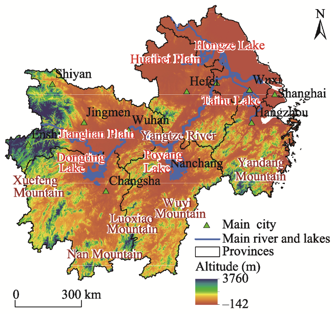
Fig. 1 The location and altitude of the study area
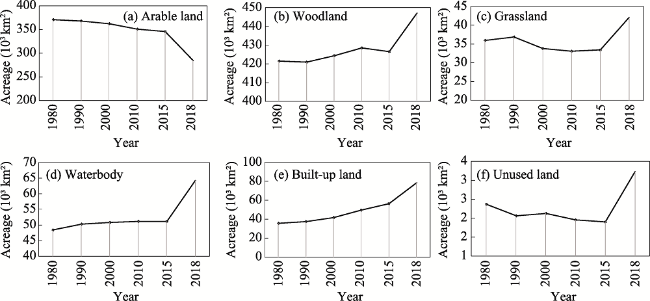
Fig. 2 Changes in each land use type in the middle and lower reaches of the Yangtze River from 1980 to 2018
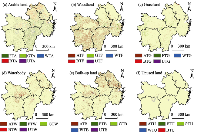
Fig. 3 Spatial distribution of land use conversions of each different land type in the middle and lower reaches of the Yangtze River from 1980 to 2018

Note: In the legend, ‘T’ is ‘transform to’; ‘A’ is ‘arable land’; ‘F’ is ‘woodland’; ‘G’ is ‘grass’; ‘W’ is ‘waterbody’; ‘B’ is ‘built-up land’; ‘U’ is ‘unused land’; so for the 3-letter codes, e.g., ‘FTA’ means woodland transform to arable land.

The increasing occupation of arable land from 1980 to 2018 is conspicuous (Fig. 3b, c, e, Table l). The arable land decreased from 371.13×10³ km² in 1980 to 283.23×10³ km² in 2018, for a total change of 87.90×10³ km² (Fig. 2a). Most of the increased cultivated land was from woodland (55.77%, 38.04×10³ km²), which is mainly in the mountainous area of central China and southern Zhejiang Province (Fig. 3b, Table 5). About one-fourth (24.43%) of the increase in cultivated was from built-up land in urban areas of either the YZR Delta, Huaibei Plain, or Jianghan Plain, Dongting Lake Plain, and Poyang Lake Plain in the middle reach of the YZR (Fig. 3e, Table 5). Built-up land increased from 36.08×10³ km² in 1980 to 78.51×10³ km² in 2018, more than doubling (Fig. 2e). Most of the newly built-up area (77.17%) was converted from arable land, which is mainly in northern Anhui Province, northern Jiangsu Province, and Yangtze River Delta (Fig. 3e). The woodland increased from 421.59 ×10³ km² in 1980 to 428.58×10³ km² in 2010, with a slight decline of 1.89×10³ km² in 2015, and it then increased to 447.35×10³ km² in 2018 (Fig. 2b). Arable land and grassland contributed 53.95% and 24.56% of the increased woodland, at 38.03×10³ km² and 17.31×10³ km², respectively (Table 5). Most of these areas were distributed in the countryside or villages of central China and the south of the YZR Delta. The grassland increased from 35.99×10³ km² in 1980 to 36.89×10³ km² in 1990, then steadily decreased to 33.18×10³ km² in 2015 and increased once again to 42.15×10³ km² in 2018 (Fig. 2c). Waterbody areas contributing 38.14% of the new grassland are mainly distributed in central China, such as Dongting Lake and Poyang Lake. The waterbody increased from 48.53×10³ km² in 1980 to 63.99×10³ km² in 2018, or 15.45×10³ km² in total area increase (Fig. 2d). Most of the increased waterbody (64.03%) was converted from arable land at 19.24 ×10³ km². The unused land decreased from 2.38×10³ km² in 1980 to 1.91 × 10³ km² in 2015 and then increased to 3.24×10³ km² in 2018 (Fig. 2f). The waterbody and arable land contributed 44.48% and 24.98% of the newly increased unused land, respectively.
Table 5 Land conversion matrix from 1980 to 2018 (km2)
Land use type 1980
Arable land Woodland Grassland Waterbody Built-up land Unused land Total acreage (2018)
2
0
1
8
Arable land 166066 38037 3964 9263 16664 281 234275
Woodland 69847 276277 13978 3736 2300 84 366222
Grassland 6277 17313 9429 834 278 18 34149
Waterbody 19243 6574 1240 21225 2104 890 51276
Construction land 43454 8482 847 3439 8265 84 64571
Unused land 620 93 29 1104 42 594 2482
Total acreage (1980) 305507 346776 29487 39601 29653 1951

3.2 Land use changes from 2050 to 2100

The spatial distribution of each land use type in the future scenarios is the same as in 2018 (Fig. 4a-h), although the proportions of each land type are different. Since land use conversion in the future scenarios are similar to the types of land use conversion from 1980 to 2018, this article does not analyze them further. The grassland and unused land will decline in the future for all scenarios, especially scenarios A1B (-60.52×10³ km² for grassland, -1.76 ×10³ km² for unused lands) (Fig. 4a, b) and B2 (-59.91×10³ km² for grassland, -1.55×10³ km² for unused land) (Fig. 4g, h). In the A1B and B1 scenarios, a considerable amount of arable land near the middle of YZR, in the Han River, Xiang River, Gan River, and southern Jianghuai Plain, would be converted to woodland. Cropland in the B1 scenario (-125.66×10³ km²) (Fig. 4e, f) will be reduced more than in the A1B scenario (-104.02×10³ km²). Correspondingly, the woodland in the A1B scenario (166.3×10³ km²) will be higher than in the B1 scenario (153.46×10³ km²) (Fig. 4e, f). The cropland acreage will increase from 2050 to 2100 in the A2 (65.54×10³ km²) (Fig. 4c, d) and B2 scenarios (89.02×10³ km²) (Fig. 4g, h). There is also an increase in build-up land from 2050 to 2100 in the A2 scenario (22.55×10³ km²) and the B2 scenario (0.88×10³ km²). Correspondingly, the woodland in the A2 scenario (-47.34×10³ km²) and the B2 scenario (-28.44×10³ km²) would decrease by 2100.
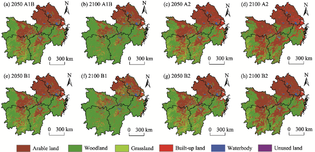
Fig. 4 Spatial distribution of land use types in the middle and lower reaches of the Yangtze River from 2050 to 2100 for four scenarios: (a,b) A1B, (c,d) A2, (e,f) B1, and (g,h) B2.

3.3 Habitat quality changes from 1980 to 2018

Many factors influence habitat quality, including human activities and physical geography. The results of the relationship analysis (Table 6) show that slope (R = 0.502, P < 0.01, in 2015), elevation (R = 0.003, P < 0.05, in 2015), population density (R = -0.299, P < 0.01, in 2015), and NDVI (R = 0.366, P < 0.01, in 2015) in the study area are significantly correlated with habitat quality (Table 4). However, the GDP and slope direction in the study area did not relate to the habitat quality. The steeper and higher an area was, the lower the population density; and the more plants there were, the higher the quality of that habitat. The relationship coefficients between these factors and habitat quality have dropped from 2000 to 2015.
Table 6 The relations between habitat quality and its impact factors from 2000 to 2015
Year Slope Aspect Altitude Population GDP NDVI
2000 0.509** - 0.0101* -0.302** - 0.369**
2010 0.501** - 0.0036* -0.296** - 0.365**
2015 0.502** - 0.003* -0.299** - 0.366**

Note: - correlation is not significant; ** correlation is significant at the 0.01 level (2-tailed); * correlation is significant at the 0.05 level (2-tailed).

The places with higher habitat quality were in the mountainous areas, especially in Yandang Mountain in southern Zhejiang, Dabie Mountain, Huang Mountain in Anhui Province, Wudang Mountain in western Hubei, Wuling Mountain in western Hunan, Xuefeng Mountain and southern South Ling and southern Jiangxi Province. The regions with lower habitat quality were distributed in the urban built-up areas, including Shanghai and Hangzhou in the Yangtze River Delta, Nanjing and Hefei in the north of lower Yangtze River, and Nanchang, Wuhan, Changsha in the middle of the Yangtze River. The habitat quality of the countryside near metropolitan areas gradually deteriorated (Fig. 6). In the first two decades, areas with low habitat quality were distributed as dots (Fig. 6a, b). With the ongoing construction of transportation and other infrastructures, more and more construction land threatened the habitat. As a result, the distribution pattern of the areas with low habitat quality gradually developed into a network, especially in the Yangzte River Delta (Fig. 6c, d, e).
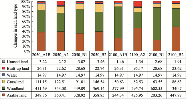
Fig. 5 Changes in each land type in the middle and lower reaches of the Yangtze River from 2050 to 2100 (´10³ km²)
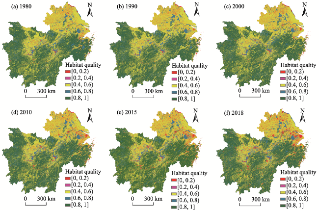
Fig. 6 Spatial-temporal distribution of habitat quality in the middle and lower reaches of the Yangtze River from 1980 to 2018
The habitat quality of each province decreased from 1980 to 2018, except for Zhejiang Province in 2018 (Fig. 7). The average values of habitat quality in Shanghai and Jiangsu were lower than those in other provinces. Jiangxi Province has the highest habitat quality among the provinces, followed by Hubei Province.
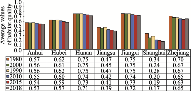
Fig. 7 Average values of habitat quality in each of the study area provinces from 1980 to 2018
To visualize the changes in habitat quality of this study area, we derived the change in habitat quality using the “raster calculator” function of ArcGIS 10.7. We subtracted the later period habitat quality from the former period habitat quality, classified the results into 10 classes of equal intervals (5 classes for negative, 5 classes for positive), and summarized the proportions of land in each class (Fig. 8, Fig. 9).
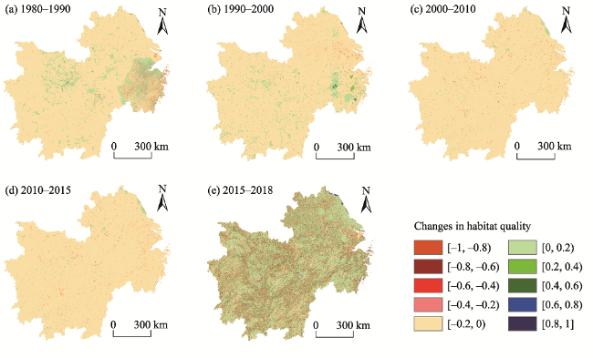
Fig. 8 Spatial distribution of changes in habitat quality in the middle and lower reaches of the Yangtze River during different time segments from 1980 to 2018
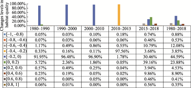
Fig. 9 The proportions of areas with different change levels in habitat quality in the middle and lower reaches of the Yangtze River from 1980 to 2018
From 1980 to 2018, 61.93% of the study area experienced habitat degradation; while 38.07% of the study area experienced habitat improvement (Fig. 8, Fig. 9). From 1980 to 1990, the degraded habitat area accounted for 91.95% of the study area, which declined in value by less than -0.2. Only 6.65% of the study area experienced an increase in habitat quality, mainly in the lower reaches of the YZR, including Taihu Lake in Jiangsu Province, Yandang Mountains in southern Zhejiang Province, Huang Mountain and Chao Lake in Anhui Province, Hanjiang Plain in Hubei Province, and Poyang Lake Plain in Jiangxi Province (Fig. 8a, Fig. 9). From 1990 to 2000, the habitat quality of 96.48% of the study areas declined by less than -0.2, and only 3.05% of the areas had a rise in habitat quality (Fig. 8c, Fig. 9). The region with improved habitat quality was clustered in Yandang Mountain in Zhejiang, Huangshan in Anhui, and Hongze Lake in Jiangsu. The habitat quality of a few places in the central YZR also increased, but they were not clustered. At this time, the decline in habitat quality in the middle and lower reaches of the YZR became accelerated, and habitat quality values fell by more than 0.4 in some eastern coastal areas. From 2000 to 2010, 96.90% of the study area experienced a decline in habitat quality, but the decline was not less than -0.2, and only 2.21% of the places experienced habitat improvement (Fig. 8c, Fig. 9). From 2010 to 2015, the declining habitat quality value of 97.56% of the areas ranged from -0.4 to -0.2. Only 0.11% of the area, distributed in the coastal land in the northeast of Jiangsu and near the river basins of those provinces, experienced improved habitat quality (Fig. 8d, Fig. 9). From 2015 to 2018, the places which experienced habitat degradation accounted for 46.13% of the study area—and places where habitat quality increased were interspersed with degraded habitat areas (Fig. 8e, Fig. 9).

3.4 Habitat quality changes from 2050 to 2100

The habitat quality of the study area shows continuing decline at a variable rate (Fig. 10). At the beginning of the two decades, its decrease was relatively slower. It declined by -0.04% per year from 1980 to 1990 and by -0.01% per year from 1990 to 2000. However, as economic growth continued, ecological degradation became more rapid, at -0.10% per year from 2000 to 2010 and -0.14% per year from 2010 to 2015. The habitat quality decreased by -0.10% per year from 2015 to 2018. By 2100, the study area's habitat quality will improve under the A1B and B1 scenarios, but it will decrease under the A2 and B2 scenarios. In conclusion, the habitat quality of the study area would be the highest under the B1 scenario, and would be the lowest under the A2 scenario.
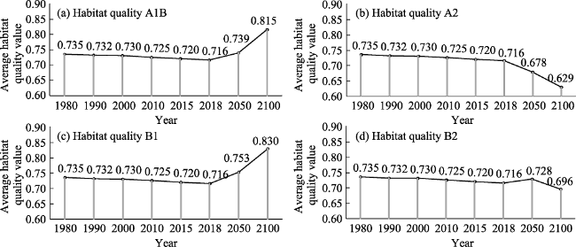
Fig. 10 Changes in the average habitat quality value in the middle and lower Yangtze River from 1980 to 2100 under the four different scenarios
Under any of the scenarios, habitat quality degradation was greater in the lower or northern YZR than in the midstream or southern areas. The habitat quality in the north of YZR is worse than in the south of YZR. The habitat quality in the plain is worse than in the mountainous areas (Fig. 11). The area with habitat quality below 0.6 is distributed in the plains, including the Lianghuai Plain of northern Jiangsu Province and northern Anhui Province, the Dongting Lake Plain of the northeastern Hunan Province, the Jianghan Plain, the Han River of the east Hubei Province, and the Poyang Lake of the north Jiangxi Province. Habitat quality under the A2 scenario (Fig. 11c, d) is the worst compared to other scenarios, followed by the B2 scenario (Fig. 11g, h). Under the A2 scenario, the habitat quality score of most of the Yangtze River Delta region is below 0.2. A rapid decline occurred in the quality of the human environment in urban and peri-urban areas. Areas of low habitat quality are distributed in networks. The habitat quality score in the B1 scenario (Fig.11e, f) is the highest compared to other scenarios, followed by the A1B scenario (Fig. 11a, b). In the A1B and B1 scenarios, the habitat quality in a few regions will increase from 2050 to 2100, and the increase interval is [0.2, 0.6] (Fig. 12a, c). The areas with increased habitat quality in these two scenarios are mainly clustered in the rivers, the lakes and their surrounding areas, such as the Han River and Jing River in Hubei, the Dongting Lake, Xiang River, Zishui, Yuan River in Hunan Province, and the Poyang Lake and Gan River in Jiangxi Province. The habitat quality of other places will decrease at a low rate.
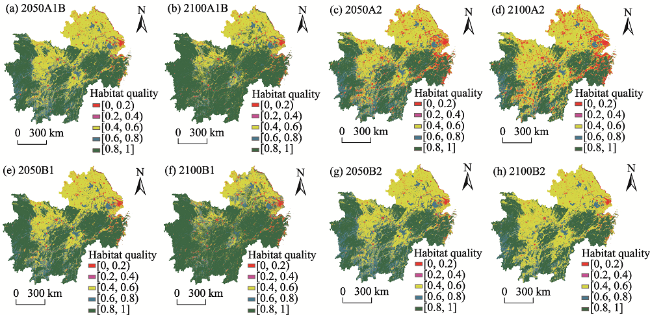
Fig. 11 Spatial distribution of habitat quality in the middle and lower Yangtze River in 2050 and 2100 under different scenarios (A1B, A2, B1, B2)
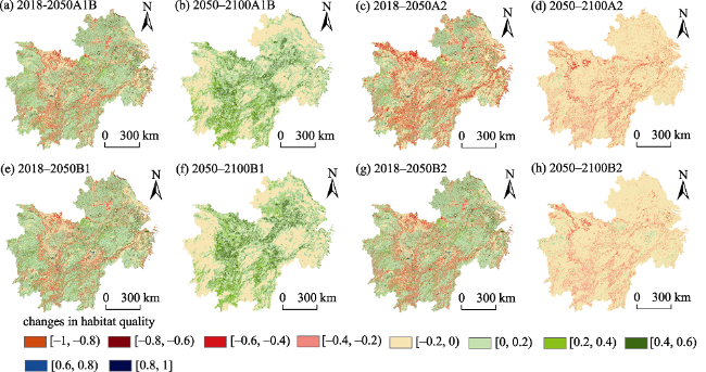
Fig. 12 Spatial distribution of changes in habitat quality in the middle and lower Yangtze River in 2100 for different scenarios (A1B, A2, B1, B2)

4 Discussion

In this study, we quantified the relationships among habitat quality, geophysical background, and human activities. The results show that the slope, elevation, population density, and vegetation cover of the terrain were significantly correlated with the quality of habitat in this study area. Forest, grasslands, and unused lands are widely distributed in the mountainous areas where vegetation cover and altitude are higher with lower population density and higher habitat quality, such as in the western Hubei Province and western Hunan Province, the border of Hubei, Hunan, and Jiangxi, southeastern mountainous areas of Zhejiang Province and southern Anhui Province. The plain areas faced considerable habitat degradation, where deforestation occurred and the arable land was converted to built-up land, and are mainly distributed in the Dongting lake Plain, Jianghan river Plain, Poyang lake Plain, northern of lower YZR.
Policies are always the key factor impacting land use modes and ecological systems. The government should pay more attention to the development of environmentally friendly policies. Areas similar to the Yangtze River have also experienced habitat degradation due to urbanization and industrialization. For example, the Ganges River in northern India (Gupta et al., 2012), Sacramento-San Joaquin Delta in the United States (Monsen et al., 2007), Lwiro River in the Democratic Republic of Congo (Bagalwa, 2006), and the River Nile in Egypt (Fishar and Williams, 2008; Chen, 2019) are all facing habitat degradation because of unsustainable land use activities and environmental pollution by industries.
Combining the results of this study with historical policies in China, we know several things: 1) The arable land protection policy (2003) curbed the decreasing rate of cropland loss. It was evident that some of the built-up land in high population density areas had changed to cropland (Fig. 3a) (Xu et al., 2015), although the increase in cultivated areas was far less than the decline in cultivated areas (Fig. 2a, e). 2) The Sloping Land Conversion Program (SLCP, also known as “Grain for Green”) was launched together with Natural Forest Protection Program (2001). Those projects worked by compensating farmers for retiring part of their land from cultivation and restoring it to either forest or grassland. Those policies resulted in a large amount of arable land being converted to woodland and an increase in local habitat quality (Fig. 2b, Fig. 3b, Fig. 7). 3) After the flooding disasters in the Yangtze River in 1998, the government launched a series of projects for returning arable lands to lakes, especially in central China (Fig. 3d, Fig. 7). These projects enlarged the lakes and adjusted the ecological environment, which had a positive effect on local habitat quality. 4) The reforming and opening-up policies of China (1980) led to a boom in the economy. An increasing amount of cropland was converted to residential houses, commercial buildings, and transportation infrastructure. The urban expansion degraded the habitat quality, especially in YZR Delta and cities located in important transportation hubs in the YZR, such as Shanghai City, urban clusters around Hangzhou in Zhejiang Province, urban clusters around Nanjing in Jiangsu Province, urban clusters around Hefei in Anhui Province, urban clusters around Wuhan in Hubei Province, the Changsha-Zhuzhou-Xiangtan City group in Hunan Province, and urban clusters around Poyang Lake in Jiangxi Province (Fig. 2, Fig. 3e). 5) After the revised and implemented Environmental Protection Law of the People’s Republic of China (2015), the environmental improvement was accelerated, which was represented by the increases in the water body, woodland, and grassland (Fig. 2).
The environmental projects converted farmland to forests and grasslands, prevented soil erosion, and maintained waterbodies, which are essential for preventing ecological degradation. Global land degradation and climate changes have been severe problems for a long time. Governments around the world should put more emphasis on ecological restoration projects for regional development, promote regional cooperation based on local conditions, optimize the regional division of labor, and construct an ecological compensation mechanism between ecologically protected areas and beneficiary areas.

5 Conclusions

In this study, we assessed the habitat quality changes from 1980 to 2100 and analyzed the influencing factors in the middle and lower reaches of the YZR, China. We found that: 1) Slope, altitude, and NDVI in the study area are significantly positively correlated with habitat quality, while the population density negatively affected the habitat quality. Moreover, the direction of slope and GDP are not significantly correlated with the habitat quality in the middle and lower reaches of YZR. 2) The habitat quality in the middle and lower reaches of the YZR has shown a downward trend over the years. Zhejiang Province is the only province where habitat quality has improved from 2015 to 2018. 3) The habitat quality in the south of the YZR is better than in the north. Environmental protection programs have mitigated local habitat quality degradation. Nevertheless, the negative impacts of urbanization on habitat quality have surpassed the positive effects of environmental protection programs. 4) If the society makes no efforts to suppress the population explosion and to suppress the expansion of construction land, to use clean energy, to accelerate energy-saving technological innovation, and to restore the ecological environment, habitat quality will worsen (particularly in the A2 and B2 scenarios). To prevent the ecological disaster caused by the loss of biodiversity, the implementation of environmental protection policies, along with environmental conservation and restoration programs, must be rigid.
This research could provide a scientific reference for wildlife protection. However, there are limitations in this study due to data constraints. For example, we did not consider water pollution in the YZR Basin, which affects the habitat quality, especially in the lower reaches of the YZR. In addition, we used a coarse land use classification to make the historical land use data consistent with future land use scenarios. The impacts of different types of land on habitat quality may vary. Cultivated land, paddy fields and dry land, construction in urban land, rural land, and industrial and mining land have different impacts on biodiversity and vary in their sensitivities to threats. Further studies could enhance the accuracy of the assessments and predictions with greater spatial resolution.
[1]
Abbott B W, Bishop K, Zarnetske J P, et al. 2019. Human domination of the global water cycle absent from depictions and perceptions. Nature Geoscience, 12(7):533-540.

DOI

[2]
Amato K R, Yeoman C J, Kent A, et al. 2013. Habitat degradation impacts black howler monkey (Alouatta pigra) gastrointestinal microbiomes. The ISME Journal, 7(7):1344-1353.

DOI PMID

[3]
Bagalwa M. 2013. The impact of land use on water quality of the Lwiro River, Democratic Republic of Congo, Central Africa. African Journal of Aquatic Science, 31(1):137-143.

DOI

[4]
Barter M, Cao L, Lei G, et al. 2006. WWF-China waterbird surveys in the lower Yangtze floodplain in 2004 and 2005. Threatened Waterfowl Specialist Group News, 88.

[5]
Aneseyee A B, Noszczyk T, Soromessa T, et al. 2020. The InVEST habitat quality model associated with land use/cover changes: A qualitative case study of the winike watershed in the Omo-gibe Basin, Southwest Ethiopia. Remote Sensing, 2(7):1103. DOI: 10.3390/rs12071103.

[6]
Chen Z Y. 2019. A brief overview of ecological degradation of the Nile Delta: What we can learn. In: Coasts and Estuaries. DOI: 10.1016/B978-0-12-814003-1.00013-7.

[7]
Chu L, Sun T, Wang T, et al. 2018. Evolution and prediction of landscape pattern and habitat quality based on CA-Markov and InVEST model in Hubei section of Three Gorges Reservoir Area (TGRA). Sustainability, 10(11):3854. DOI: 10.3390/su10113854.

DOI

[8]
Dai L, Li S, Lewis B J, et al. 2019. The influence of land use change on the spatial-temporal variability of habitat quality between 1990 and 2010 in Northeast China. Journal of Forestry Research, 30(6):2227-2236.

DOI

[9]
Erdozain M, Thompson D, Porter T M, et al. 2019. Metabarcoding of storage ethanol vs. conventional morphometric identification in relation to the use of stream macroinvertebrates as ecological indicators in forest management. Ecological Indicators, 101:173-184.

DOI

[10]
Fishar M R, Williams W P. 2008. The development of a Biotic Pollution Index for the River Nile in Egypt. Hydrobiologia, 598(1):17-34.

DOI

[11]
Gaffin S R, Xing X, Yetman G. 2002. Country-level GDP and downscaled projections based on the SRES A1, A2, B1, and B2 marker scenarios, 1990-2100. Palisades, NY: NASA Socioeconomic Data and Applications Center (SEDAC).

[12]
Gupta B K, Sarkar U K, Bhardwaj S K. 2012. Assessment of habitat quality with relation to fish assemblages in an impacted river of the Ganges basin, northern India. The Environmentalist, 32(1):35-47.

DOI

[13]
Hack J, Molewijk D, Beißler M R. 2020. A conceptual approach to modeling the geospatial impact of typical urban threats on the habitat quality of river corridors. Remote Sensing, 12(8):1345. DOI: 10.3390/ rs12081345.

DOI

[14]
Jiang W, Deng Y, Tang Z, et al. 2017. Modelling the potential impacts of urban ecosystem changes on carbon storage under different scenarios by linking the CLUE-S and the InVEST models. Ecological Modelling, 345:30-40.

DOI

[15]
Johnson M D. 2007. Measuring habitat quality: A review. The Condor, 109(3):489-504.

DOI

[16]
Li X, Hou X, Song Y, et al. 2019. Assessing changes of habitat quality for shorebirds in stopover sites: A case study in Yellow River Delta, China. Wetlands, 39(1):67-77.

DOI

[17]
Liang W, Yang M. 2019. Urbanization, economic growth and environmental pollution: Evidence from China. Sustainable Computing: Informatics and Systems, 21:1-9.

[18]
Liu J, Liu M, Zhuang D, et al. 2003. Study on spatial pattern of land-use change in China during 1995-2000. Science in China Series D: Earth Sciences, 46(4):373-384.

[19]
Liu X, Liang X, Li X, et al. 2017. A future land use simulation model (FLUS) for simulating multiple land use scenarios by coupling human and natural effects. Landscape and Urban Planning, 168:94-116.

DOI

[20]
Liu Y, Zhou Y, Du Y. 2019. Study on the spatio-temporal patterns of habitat quality and its terrain gradient effects of the middle of the Yangtze River Economic Belt based on InVEST model. Resources and Environment in the Yangtze Basin, 28(10):2429-2440. (in Chinese)

[21]
Manangkalangi E, Rahardjo M F, Hadiaty R K, et al. 2019. Distribution and abundance of the arfak rainbowfish, Melanotaenia arfakensis Allen, 1990 in Prafi River system, Manokwari, West Papua: Due to habitat degradation? IOP Conference Series: Earth and Environmental Science, 12-43.

[22]
Monsen N E, Cloern J E, Burau J R. 2007. Effects of flow diversions on water and habitat quality: Examples from California’s highly manipulated Sacramento—San Joaquin Delta. San Francisco Estuary and Watershed Science, 5(5):1-16.

[23]
Nadakavukaren A, Caravanos J. 2020. Our global environment: A health perspective. Long Grove, USA: Waveland Press.

[24]
Nakicenovic N, Alcamo j, Grubler A, et al. 2000. Special report on emissions scenarios (SRES), a special report of Working Group III of the intergovernmental panel on climate change. Cambridge, UK: Cambridge University Press.

[25]
Nelson E, Mendoza G, Regetz J, et al. 2009. Modeling multiple ecosystem services, biodiversity conservation, commodity production, and tradeoffs at landscape scales. Frontiers in Ecology and the Environment, 7(1):4-11.

DOI

[26]
Niemi G J, McDonald M E. 2004. Application of ecological indicators. Annual Review of Ecology, Evolution, and Systematics, 35:89-111.

[27]
Öckinger E, Dannestam Å, Smith H G. 2009. The importance of fragmentation and habitat quality of urban grasslands for butterfly diversity. Landscape and Urban Planning, 93(1):31-37.

DOI

[28]
Pettorelli N, Gaillard J, Duncan P, et al. 2001. Population density and small-scale variation in habitat quality affect phenotypic quality in roe deer. Oecologia, 128(3):400-405.

DOI PMID

[29]
Powers R P, Jetz W. 2019. Global habitat loss and extinction risk of terrestrial vertebrates under future land-use-change scenarios. Nature Climate Change, 9(4):323-329.

DOI

[30]
Pulliam H R. 2000. On the relationship between niche and distribution. Ecology Letters, 3(4):349-361.

DOI

[31]
Rao C S, Kareemulla K, Krishnan P, et al. 2019. Agro-ecosystem based sustainability indicators for climate resilient agriculture in India: A conceptual framework. Ecological Indicators, 105:621-633.

DOI

[32]
Smith J L D, Ahearn S C, McDougal C. 1998. Landscape analysis of tiger distribution and habitat quality in Nepal. Conservation Biology, 12(6):1338-1346.

DOI

[33]
Sharp R, Tallis H T, Ricketts T, et al. 2018. InVEST 3.7.0. user’s guide. The Natural Capital Project.

[34]
Upadhaya S, Dwivedi P. 2019. Conversion of forestlands to blueberries: Assessing implications for habitat quality in Alabaha river watershed in Southeastern Georgia, United States. Land Use Policy, 89:104229. DOI: 10.1016/j.landusepol.2019.104229.

DOI

[35]
Van H B. 1983. Density as a misleading indicator of habitat quality. The Journal of Wildlife Management, 47(4):893-901.

[36]
Wang H, Tang L, Qiu Q, et al. 2020. Assessing the impacts of urban expansion on habitat quality by combining the concepts of land use, landscape, and habitat in two urban agglomerations in China. Sustainability, 12(11):4346. DOI: 10.3390/su12114346.

DOI

[37]
Whittington J, Low P, Hunt B. 2019. Temporal road closures improve habitat quality for wildlife. Scientific Reports, 9(1):1-10.

PMID

[38]
Xu G, Huang X, Zhong T, et al. 2015. Assessment on the effect of city arable land protection under the implementation of China’s National General Land Use Plan (2006-2020). Habitat International, 49:466-473.

DOI

[39]
Xu L, Chen S S, Xu Y, et al. 2019. Impacts of land-use change on habitat quality during 1985-2015 in the Taihu Lake Basin. Sustainability, 11(13):1-21.

DOI

[40]
Zhang X, Zhou J, Li G, et al. 2020. Spatial pattern reconstruction of regional habitat quality based on the simulation of land use changes from 1975 to 2010. Journal of Geographical Sciences, 30(4):601-620.

DOI

[41]
Zhong L, Wang J. 2017. Evaluation on effect of land consolidation on habitat quality based on InVEST model. Transactions of the Chinese Society of Agricultural Engineering, 33(1):250-255.

[42]
Zhou B, Yu X, Chen L, et al. 2010. Soil erosion simulation in mountain areas of Beijing based on InVEST model. Research of Soil and Water Conservation, 17(6):9-13.

[43]
Zhou S, Zhang M. 2011. An integrated analysis into the causes of ungulate mortality in the Wanda Mountains (Heilongjiang Province, China) and an evaluation of habitat quality. Biological Conservation, 144(10):2517-2523.

DOI

[44]
Zhu C, Zhang X, Zhou M, et al. 2020. Impacts of urbanization and landscape pattern on habitat quality using OLS and GWR models in Hangzhou, China. Ecological Indicators, 117:106654. DOI: 10.1016/ j.ecolind.2020.106654.

DOI

Outlines

/