Animal Ecology

Study of Vulture Habitat Suitability and Impact of Climate Change in Central India Using MaxEnt

  • Kaushalendra K. JHA , 1, * ,
  • Radhika JHA 2
Expand
  • 1. Indian Institute of Forest Management, Nehru Nagar, Bhopal, Madhya Pradesh 462003, India
  • 2. Department of Zoology, University of Lucknow, Lucknow, Uttar Pradesh 226007, India
*Kaushalendra K. JHA, E-mail:

Received date: 2020-06-16

  Accepted date: 2020-08-15

  Online published: 2021-03-30

Abstract

Vultures provide invaluable ecosystem services and play an important role in ecosystem balancing. The number of native vultures in India has declined in the past. Acquiring present knowledge of their habitat spread is essential to manage and prevent such a decline. It is envisaged that ongoing climate crisis may further cause change in habitat suitability and impact the existing population. Therefore, this study in Central India—a vulture stronghold, is aimed at predicting habitat changes in the short and long term and present the data statistically and graphically by using Species Distribution Model. MaxEnt software was chosen for its advantages over other models, like using presence-only data and performing well with incomplete data, small sample sizes and gaps, etc. Global Climate Model ensemble (CCSM4, HadGEM2AO and MIROC5), was used to get better prediction. Fourteen robust models (AUC 0.864-0.892) were developed using data from over 1000 locations of seven vulture species over two seasons together. Selected climatic and other environmental variables were used to predict the current habitat. Future prediction was based on climatic variables only. The most important variables influencing the distribution were precipitation (bio 15, bio 18, bio 19) and temperature (bio 3, bio 5). Forest and water bodies were the major influencers within land use-landcover in the current prediction. At finer scale, while extremely suitable habitat area decreased and highly suitable area increased over time, the total suitable area marginally increased in 2050 but decreased in 2070. For broader consideration, net loss in suitable area was 5% in 2050 and 7.17% in 2070 (RCP4.5). Similarly, in the RCP8.5 this was 6% in 2050 and 7.3% in 2070. The data generated can be used in conservation planning and management and thus protecting the vultures from any future threat.

Cite this article

Kaushalendra K. JHA , Radhika JHA . Study of Vulture Habitat Suitability and Impact of Climate Change in Central India Using MaxEnt[J]. Journal of Resources and Ecology, 2021 , 12(1) : 30 -42 . DOI: 10.5814/j.issn.1674-764x.2021.01.004

1 Introduction

Throughout the world, scavenger birds are declining rapidly with some populations already on the brink of extinction (Straub et al., 2015). Vultures are the only obligatory scavengers among all raptors, worthy of paramount ecological importance. Among them, old world vultures are the most threatened group (McClure et al., 2018). Any threat to them leads to a disbalance of ecological equilibrium carrying risks of pollution and diseases in wildlife, humans and livestock. Seven old world vultures [Egyptian Vulture (Neophron percnopterus) (EV), Indian Vulture or Long-billed Vulture (Gyps indicus) (LV), White-rumped Vulture (Gyps bengalensis) (WV), Red-headed Vulture (Sarcogyps calvus) (RV), Cinereous Vulture (Aegypus monachus (CV), Eurasian Griffon (Gyps fulvus) (EG) and Himalayan Griffon (Gyps himalayensis) (HG)], out of nine species found in the wild in India (Ali and Ripley, 1987), are common to Central India, a vulture stronghold (Jha, 2018).
Between 1990s and first decade of this century, a sharp decline was reported in the population of the Gyps genus in India (Prakash et al., 2003; Anon, 2006). Further research pointed towards seven probable causes (Anon, 2004; Markandya et al., 2013). Among these, apart from the use of Diclofenac as a major cause of the decline in numbers (Prakash et al., 2007), loss of habitat also posed a crucial risk to the survival of these species. The loss and transformation of natural habitat and breeding sites (Boshoff and Vernon, 1980; Naidoo et al., 2011) has caused a decline in vulture populations in many parts of the world (Schabo et al., 2016). Therefore, this warrants a detailed study of habitat suitability and change, if any.
An organism’s habitat is the combination of the space it inhabits and all eco-factors in that space, including the abiotic environment and other organisms that are necessary for the existence of individuals or groups (Yi et al., 2016). Habitat alteration is inevitable due to climate crisis on account of continued increase in greenhouse gas emission. Change in carbon concentration as a result of anthropogenic activity is predicted to change the temperature and precipitation patterns in the years to come which could change the spread of vulture habitat. The studies should be centred around bioclimatic variables, such as temperature and precipitation and their ranges as well as environmental ones, such as topography (elevation, slope aspect, water bodies etc.) and land use-landcover of the region influencing the vulture population. A habitat suitability index (HSI), which is a probability of species presence inferred from ecological niche modelling, by relating the occurrence of a species at a given location to environmental features (Guisan and Thuiller, 2005), can be developed for the same demarcating the area from most suitable to least suitable. This can be achieved by various Species Distribution Models (SDMs) which extrapolate presence and absence data and identify similar areas of interest. One such widely used presence-based classical and reliable SDM is MaxEnt which has several advantages over others. Among several SDMs, MaxEnt modelling has been widely employed, because it performs well with either incomplete data or presence-only data (Phillips et al., 2006). This model has been equally applied to both plant and animal conservation (Phillips et al., 2006; Zhang et al., 2018), apart from endangered species management (Ashraf et al., 2016).
In the context of the above facts, this paper aims to (i) map the current distribution of the habitat of vultures, (ii) categorise the habitat suitability using HSI and (iii) predict and map the future habitat impacted by climate change in Central India, using MaxEnt.

2 Materials and methods

2.1 Study area

Central India, Madhya Pradesh (21°06′-26°30′N, 74°00′-82°51′E) was chosen for this study as it has the maximum number of locations (roosting/breeding sites), vulture species and individuals compared to other states of India (Jha, 2018). It has a varied topography of plateaus, hills, and valleys supporting agricultural areas, forest areas and interspersed waterbodies. The temperature and rainfall range from 1 ℃ to 47 ℃ and 1000 mm to 2150 mm, respectively. The state is covered under three climatic regions of India—semi-arid in north west, tropical wet and dry in south west, and sub- tropical wet and dry in the remaining, much larger part. These regions have dominance of open forest (>10%) and scrub, very dense forest (>70%) and moderately dense forest (>40%), respectively, in terms of canopy cover.
2.1.1 Species and presence data
Vulture presence data was recorded once each in the winter and summer of 2016 (Jha, 2017) from over 1000 locations comprising roosts and nests of seven vulture species sighted during the census. Head count was done by similarly skilled teams of two persons each covering three to four sites out of all historically/currently identified locations on a pre- decided single date. Garmin GPS was used to record the locations of vulture sightings. This was plotted on the map of central India using ArcGIS software (Fig. 1, adopted from Jha et al., 2020). Vulture species located in the study could be grouped as resident: LV, WV, RV and EV and migratory: CV, EG and HG. The former group used the habitat for nesting and roosting while the latter for roosting only for few months. All the locations were combined for vulture habitat assessment in the study area.
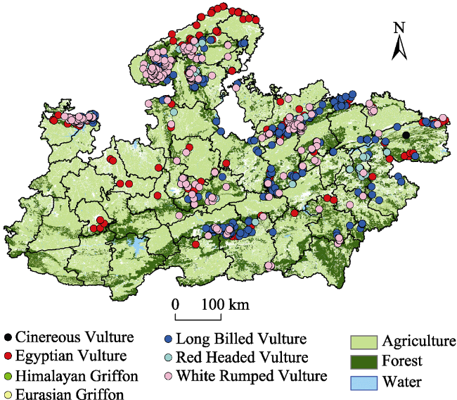
Fig. 1 Location of vulture species in Central India surveyed in 2016

Note: This presence only record has been used in Species Distribution Model, MaxEnt, as sample input. Proximity of vulture locations may be noted to forested landscape in most cases.

2.1.2 Environmental variable selection
Distribution of any species depends on variables related to climate and it is likely that the species could rapidly respond to climatic change (Luoto et al., 2006). Keeping this in view, 19 bioclimatic variables were downloaded from worldclim.org. Other environmental variables were also included in order to increase the accuracy of the habitat prediction (Jha and Jha, 2020), since the reliability of species distribution modelling is based on selecting ecologically relevant environmental predictors (Elith and Leathwick, 2009). Land use-landcover (LULC), especially the trees/forests and mountain cliffs directly influence vulture habit, while elevation and aspect have an indirect influence. Lofty trees in open forest (Thakur and Narang, 2012; Ramkrishnan et al., 2014) and high cliffs (Mateo-Tomas and Olea, 2009; Campbell, 2015) are used for nest building. Non-Differential Vegetation index (NDVI) is an indirect indicator of food availability (Santangeli et al., 2018) and southern aspect is the preferable direction (Liberatori and Penteriani, 2001; Sen et al., 2017).
However, correlations between the bioclimatic variables could lead to poor model performance affecting the result (Angelieri et al., 2016; Abolmaali et al., 2018, Ahmad et al., 2019). Therefore, to eliminate collinearity, Pearson’s correlation analysis was performed setting the coefficient threshold at ±0.8 (Yang et al., 2013; Ashraf et al., 2016; Cao et al., 2016; Abolmaali et al., 2018). Thus, extracted non-colinear variables used in the SDM is presented in Table 1.
Table 1 Selected variables used in vulture habitat prediction model
Bio-climatic Environmental
Temperature Precipitation
(i) bio 3 = Isothermality (bio 2/bio 7) ×100 (v) bio 13 = Precipitation of wettest month (x) LULC (Forest, water, rural and urban built-up area, agriculture, wasteland, scrubland)
(ii) bio 5 = Max temperature of warmest month (vi) bio 14 = Precipitation of driest month (xi ) NDVI (January 2016)
(xii) NDVI (May 2016)
(iii) bio 9 = Mean temperature of driest quarter (vii) bio 15 = Precipitation seasonality
(coefficient of variation)
(xiii) Elevation
(iv) bio 11 = Mean temperature of coldest quarter (viii) bio 18 = Precipitation of warmest quarter
(ix) bio 19 = Precipitation of coldest quarter
2.1.3 Climate model and pathway selection
There are different Global Circulation Models (GCMs) and Representative Concentration Pathways (RCP2.6, RCP4.5, RCP6.0, RCP8.5) representing the bioclimatic variables and climate scenarios (Meinshausen et al., 2011; Stocker, 2014). Since there is no consensus as to what makes the most accurate GCM, integrating different GCMs and RCPs to reinforce accuracy of the projections is strongly recommended (Sutton et al., 2015). Such ensemble modelling is a very common approach for habitat projection in plants and animals (Ng et al., 2018; Stiels and Schidelko, 2018). We chose commonly used GCMs like, CCSM4 (Shabani et al., 2018; Abdelaal et al., 2019; de Luis et al., 2019, etc.), HadGEM2AO (Ahmad et al., 2018; Shabani et al., 2018), MIROC5 (Sony et al., 2018; Shabani et al., 2018), among 17 available CMIP5 GCMs (Hayes and Piaggio, 2018) and two RCPs namely, Moderate RCP4.5 and Extreme RCP8.5 (de Luis et al., 2019; Dew et al., 2019) for short-term (year 2050) and long-term prediction (year 2070) based on the hypothesis that a sharp cut in CO2 emission will not happen (Lane, 2018) and lower emission scenarios will be rather unlikely (Manning et al., 2010). Model averaging was done in order to increase prediction accuracy (Dormann et al., 2018).
2.1.4 Species distribution modelling
Species distribution models are becoming an increasingly popular tool in ecology as they help establish relationships between the geographical location of a species and its environmental and climatic conditions (Kumar and Stohlgren, 2009). Maxent (Jafari et al., 2016; McDonald et al., 2019) SDM, hereafter MaxEnt (Elith et al., 2011; Abdelaal et al., 2019), version 3.4.1 was used in this study. This is a machine learning algorithm that allows SDMs to be generated. It is one of the most reliable and statistically robust modelling softwares among well-established SDMs (Phillips et al., 2004, 2006; Elith et al., 2006; Wisz et al., 2008). It is also the most frequently used method for SDM/ENM and has been shown to perform better than many other models (Phillips et al., 2006; Elith et al., 2006; Banag et al., 2015). It has become the most popular modelling tool for both its ease of use and functionality (Morales et al., 2017; Mohammadi et al., 2019). This could be due to its higher predictive accuracy than any other method (Elith et al., 2006; Summers et al., 2012).MaxEnt was chosen due to its primary advantages like, 1) it requires only presence data to generate the probability of presence on a scale of 0 to 1 (Kumar and Stohlgren, 2009); 2) it can work with a small sample size (Kumar and Stohlgren, 2009; Abolmaali et al., 2018); 3) it is easy to use (Angelieri et al., 2016); 4) it is very useful when presence-absence data collection is impractical (Phillips et al., 2006); 5) it outperforms other methods when the number of geographic records is scarce (Elith et al., 2006; Phillips and Dudík, 2008; Wisz et al., 2008); 6) both, categorical and continuous environmental layers can be applied in this software; 7) it is a suitable choice for prediction of distribution for rare and threatened species (Hernandez et al., 2006; Wisz et al., 2008); 8) it creates a spatially explicit map for habitat suitability with an easy interpretation; 9) it measures importance of each environmental variable using the jackknife test, in terms of gain (Elith et al., 2011; Groff et al., 2014), and 10) it can be used to project into the future under climate change to predict habitat losses and gains within species range (Phillips et al., 2006; Elith et al., 2011; Abdelaal et al., 2019).
2.1.5 Data preparation
Data, apart from vulture sighting or locations, used in this study were available at different sources and of varied resolution. To bring in uniformity among the procured data (Bioclim variables from www.worldclim.org/bioclim, NDVI and elevation from www.earthexplorer.usgs.gov) and resolution (“0.00833×0.00833” and “231.6563583×231.6563583”), file preparation was done for species presence sample, environmental variables for current and future scenario [flow chart in Fig. 2; Modified from Zhang et al. (2019) and Mwakapeje et al. (2019)].
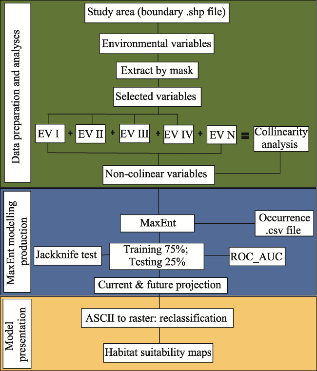
Fig. 2 Flow chart of Species Distribution Modelling using MaxEnt software

Note: EV I to EV IV are environmental variables (Table 1); N indicates any number of EV. Flow is top to bottom along connectors.

2.1.6 Habitat mapping
ArcGIS (10.3) software was used for conversion of index based MaxEnt maps to a presentable version as jpeg files. The same software was used for averaging the GCMs, habitat area calculation and identification of area suitability status. The study area was divided artificially into five categories on the basis of MaxEnt index, e.g., least suitable (0-0.2], slightly suitable (0.2-0.4], moderately suitable (0.4-0.6], highly suitable (0.6-0.8] and extremely suitable (0.8-1]. Yang et al. (2013) and Qin et al. (2017) were consulted for classifying the prediction range for suitability of habitat. For calculation of gain and loss in vulture habitat these fine scale categories were merged in to low suitable (0-0.4] and high suitable area (0.4-1].

3 Results

Relative species abundance indicated that only 2.8% of total population was migratory (CV, HG, EG). Among residents, RV contributed only 1.3%. Major contributors like, LV and EV were 47.5% and 26.5%, respectively. WV provided 21.5% individuals. On almost similar trends, residents and migratory species occupied 95% and 5% locations. LV occupied cliffs while WV preferred trees. EV was seen in cliffs as well as trees while RV on trees only. CV, HG and EG were seen roosting at either of the sites during winter months.Pearson’s coefficient test resulted in the elimination of ten colinear bioclimatic variables (bio 1, bio 2, bio 4, bio 6, bio 7, bio 8, bio 10, bio 12, bio 16 and bio 17) on ±0.8 threshold value. This ensured non-ignorance of spatial autocorrelation and multicollinearity which may lead to false ecological conclusions in modelling spatial distribution of species (de Frutos et al., 2007). Consequently, habitat prediction results were based on the remaining nine bioclimatic and four environmental variables (Table 1) in the case of current scenario while future scenarios were based on only nine bioclimatic variables due to non-availability of future LULC and NDVI data.Fourteen models were obtained as MaxEnt products. All the models were found to have AUC value more than 0.86 (0.864-0.892). Model impacting parameters were analysed using jackknife test bar chart, variable contribution estimate table and response curves. In the case of the current scenario, the former two (bar chart and table) showed that LULC was the most influential predictor (Fig. 3; top left). Contribution estimation table indicated that it was 54.6%. Response curve chart of LULC (used as categorical variable) revealed that forest and waterbody was the most while agricultural area the least important component among others including urban and rural built-up area, wasteland and scrubland.
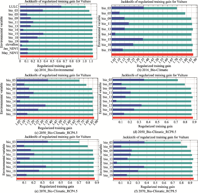
Fig. 3 Jackknife charts of variable contribution in model prediction

Note: The bars in light blue represent without variable; the bars in dark blue represent with only variable; the bars in red represent with all variables.

In the future scenario where environmental variables were not available/used, isothermality (bio 3), max temperature of warmest month (bio 5), precipitation seasonality (bio 15), precipitation of warmest quarter (bio 18), precipitation of coldest quarter (bio 19), mean temperature of driest quarter (bio 9), mean temperature of coldest quarter (bio 11), precipitation of driest month (bio 14), and precipitation of wettest month (bio 13) were found to impact the prediction in decreasing order based on average value derived from variable contribution estimate table. First five variables influenced the models around 85% while first three contributed around 68%. Jackknife results (Fig. 3) showed minor variation from this result.Different categories of habitat suitability area (HSA) were assessed and diagrammatically presented in Fig. 4 since predicting suitable habitat distribution is an effective way to protect rare or endangered species (Cao et al., 2016). HSA under different categories within two current scenarios, based on climatic variables and environmental variables are different (Table 2). Least suitable area in the environmental case is higher as compared to climatic one. Consequently, suitable area projection in the current scenario with environmental variables is lower in all the categories (by 26 km2 in highly suitable to 40580 km2 in slightly suitable).
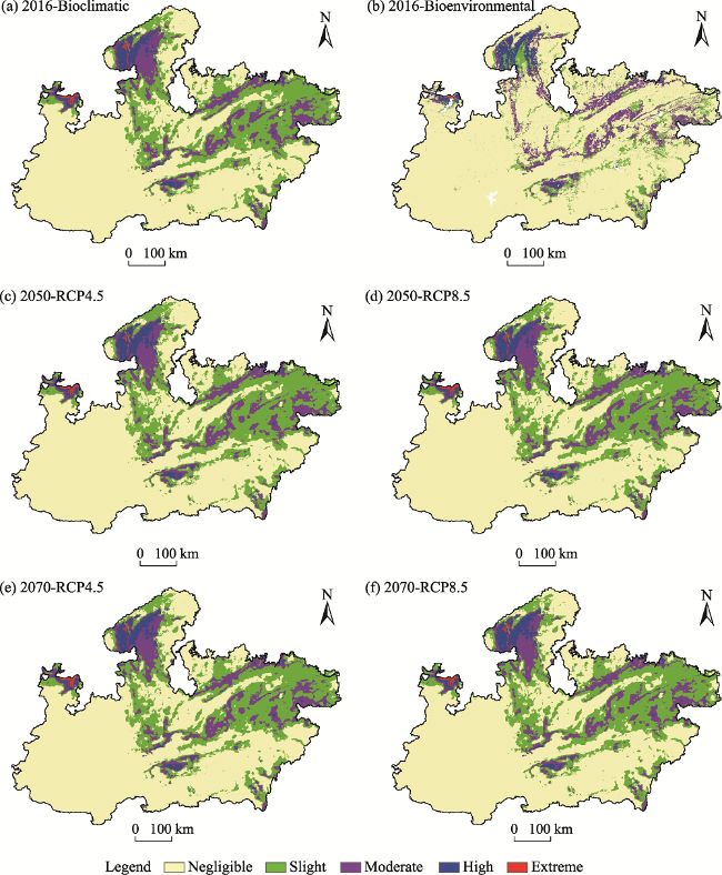
Fig. 4 The expanse of habitat suitability classes under different scenarios

Note: Top two maps compare impact of LULC inclusion in terms of reduced suitable area in the top right map.

Table 2 Habitat suitability area (km2; average of three GCMs) distribution among different categories under varied scenario
Habitat suitability category Current (2016) Short term (2050) Long term (2070)
Environmental Climatic Climatic Climatic
RCP4.5 RCP8.5 RCP4.5 RCP8.5
Least suitable 242265 (79.3) 189013 (61.1) 187442 (60.6) 188833 (61.0) 191174 (61.8) 190816 (61.7)
Slightly suitable 27733 (9.1) 78313 (25.3) 79883 (25.8) 79138 (25.6) 76827 (24.8) 78066 (25.2)
Moderately suitable 28089 (9.2) 33930 (11.0) 33347 (10.8) 33330 (10.8) 32513 (10.5) 31633 (10.2)
Highly suitable 7310 (2.4) 7336 (2.4) 8020 (2.6) 7357 (2.4) 8139 (2.6) 8118 (2.6)
Extremely suitable 217 (0.1) 829 (0.3) 729 (0.2) 764 (0.2) 769 (0.2) 788 (0.3)

Note: Figures in parentheses are percentage of the total area available.

However, the predicted suitable habitat (slight to extremely suitable) is distributed mainly in the forest with tall trees and hilly tracts covered at the top and surrounded by forest in the foothills. The adjacent area to the forest in agriculture landscape is also suitable but in limited expanse. Altitudinal significance was not obvious since hills of central India as such are not very high but strategical advantage allowed vultures to colonise on cliffs up to 200 m from the ground.
Due to inconsistency in change of different category of suitability area at finer HSI range (five classes; Table 2), reclassified area at broader HSI range (two classes; Table 3 and Fig. 5) was analysed for loss and gain in low suitability and high suitability area. In the present scenario the area with low and high suitability was estimated to be 266641 km2 and 41987 km2, respectively. Upon studying the impact of the climate crisis this area reduced in both the short term and long term except for the short-term scenario with moderate control of anthropogenic activities contribution to greenhouse gas emissions (i.e. RCP4.5 of 2050). In this case the change was found to be negligible. However, in the short- term scenario with extreme lack of control (RCP8.5 of 2050) a net loss of 673 km2 was noted. Similarly, in the long-term scenarios with moderate control (RCP4.5 of 2070) and with extreme lack of control (RCP8.5 of 2070) the net loss of area was found to be 642 km2 and 1552 km2, respectively. Percentage loss in area was found to be 5% in the short term and 7.17% in the long term in the RCP4.5 scenario. In the RCP8.5 scenario the percentage loss was found to be 6% in the short term and 7.30% in the long term.
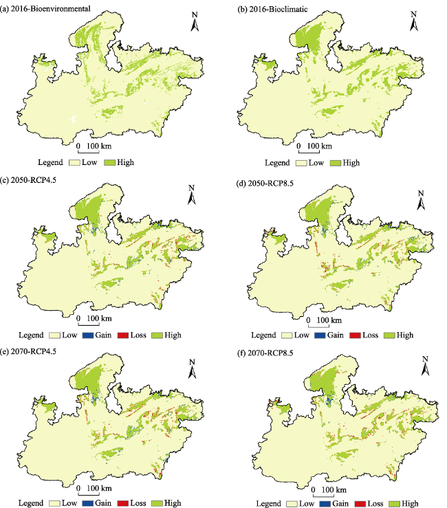
Table 3 Data representing the expanse of habitat suitability and possible future change in km2

Category
Bioclimatic RCP4.5 RCP8.5
2016 2050 2070 2050 2070
Low habitat suitability 266641 264391 264294 264599 265111
Gain 0 2250 2347 2042 1530
Loss 0 2249 3020 2685 3082
High habitat
suitability
41987 39738 38967 39302 38905
Fig. 5 The changes in vulture habitat area suitability from low to high and vice versa in short term (2050) and long term (2070) with respect to present (2016)
Current scenario compared with short-term and long- term prediction indicated that least suitable area decreased in short term but it was the opposite in long term in both RCPs. The trend was inverse in the case of slightly suitable area. Moderately suitable and extremely suitable area decreased while highly suitable area increased in all the cases in the future.

4 Discussion

Species distribution models have become increasingly important in the last few decades for the study of biodiversity, macro ecology, community ecology and the ecology of conservation. An accurate knowledge of the spatial distribution of species is of crucial importance for landscape management, preservation of rare and/or endangered species, measurement of the impact of climate change on species, etc. (Botella et al., 2018). Therefore, keeping in view these scenarios, we discuss the grouping of species and results of MaxEnt SDM for vulture distribution and habitat projection in Central India in the following paragraphs.
Occurrence probability (ψ) of vultures in the whole study area was 18.8%, while it was 3.7% in agriculture and 17.7% in forest landscape, respectively (Jha et al., 2020). Different vulture species recorded during the census were all endangered to threatened obligate scavengers using common and abundant resources like food (domestic and wild ungulates), water and shelter (forests and cliffs). Migratory being very low in number and site occupancy, including one resident (RV) was merged together with prominent but using mutually exclusive shelters like forest trees (WV) and Cliff (LV). EV was dispersed over cliff, forest trees and agriculture landscape. Jha et al. (2020) reported that residency of the total population was 87% in forest and 13% in agriculture landscape with over all density 0.02 km-2 in the study area. Holland et al. (2019) suggested that smaller migratory population could be merged with residents. Marshal et al. (2008) observed that competition remains unclear among the species probably due to abundance of resources for a limited population. Genero et al. (2020) reported dietary plasticity in vultures which may reduce competition load. Moreover, the ultimate objective of the study was to find out coarse grained information needed by the managers for conservation of these species which are more alike than different. Keeping this in view the species and ecological differences were not required to be scaled.
The preferred technique to test the accuracy of models generated for presence only data is the AUC of ROC value (Stockwell and Peters, 1999; Bosch et al., 2012). Generally, models having 0.5 AUC value are considered no better than random and AUC closer to 1 are considered perfect performers (Phillips et al., 2006; Bosch et al., 2014). Several researchers (Pearce and Ferrier, 2000; Newbold et al., 2009) recorded that AUC values above 0.9 indicate the highest accuracy of the model. Our models were robust enough to rely upon as the incorporation of static and dynamic variables returned AUC test value >0.86 which is a high predictive performance (Araújo et al., 2005). As suggested by Swets (1988), Baldwin (2009), Lv et al. (2012), etc. this value also fell in the category of good performer as classified (AUC: >0.9 = very good; AUC: 0.7-0.9 = good, AUC: <0.7 = uninformative).
Selection of parameters or predictor variables were based on literature indicating the relationship between vultures and their habitat, for example roosting and nesting places on tall trees and cliffs in and around forest (Thakur and Narang, 2012; Joshi et al., 2015; Jha et al., 2020), water requirement (Kushwaha, 2016), impact by road traffic and habitation (Bamford et al., 2009; Chomba and M’Simuko, 2013), etc. These were covered in our study under LULC (rural and urban built-up area, roads and mines, forest, waterbodies, wasteland, agriculture and scrubland). NDVI was included to cater for food availability in the region as it could be an indirect indicator of ungulate presence (Santangeli et al., 2018). January and May NDVI were taken separately as the forests in the study area are mostly deciduous and have different canopy reflectance in these two periods as a result of different structure of forests influencing vulture habit in studied area.
The important fact which can be gleaned from the results of model run is the importance and impact of different variables and the role they play in influencing the habitat of vulture species. This is represented by the Jackknife test outcome (Fig. 3). Some bioclimatic variables did play their role in habitat prediction but bioenvironmental predictors played a major share (Figs. 3-5). Gama et al. (2015), studying the impact of sets of variables on area suitability, concluded that climatic factors in isolation and in combination with environmental factors give similar predictions. But our result contradicted this as the climatic set of variables returned larger suitable area than in combination with the environmental set. This variation in findings could be the difference in the environmental set in these two studies, since the former did not include habitat limiting factors like water and vegetation. However, the reason for change in suitable area in the present study could be attributed to the fact that the climatic umbrella is mostly larger than the environmental one due to the specific requirement of a niche (trees/ cliffs, water, ungulate/ cattle concentration etc.). This is also corelated to a smaller suitable vulture area in bioenvironmental prediction (20.8%) in comparison to bioclimatic prediction (39%) in the case of the current scenario.
Climate change has been identified as a major cause of habitat loss (Kumar, 2012; Newbold et al., 2015) while habitat loss is regarded as the most important factor in the loss of biodiversity (Jiao et al., 2016; Liu et al., 2017). Habitat loss in the present case, although small (5%-6% in short term and 6%-7% in long term), is an alert signal for the future management of the conservation of these threatened vulture species. This could be a precursor to major loss in a much longer term. However, the significant drivers, other than LULC projected in the present study, are temperature and precipitation [Isothermality (bio 3), Max temperature of warmest month (bio 5), Precipitation seasonality (bio 15), Precipitation of warmest quarter (bio 18) and Precipitation of coldest quarter (bio 19)]. The latter seems to be more important than the former on the basis of field observation, wetter area (Moist deciduous forests) with less vulture locations than drier area (Dry deciduous forests) in a state where temperature variation is marginal. This is in agreement with (Tyrberg, 2010) that precipitation (changes in monsoon) may be more important for the bird community than temperature changes, particularly limited to a 2 ℃ rise. These implications may affect vultures more indirectly due to reduction in habitat area and cover composition than directly by forcing them to adapt physiologically the changed climatic conditions (Aragon et al., 2010; Sercioglu et al., 2012).
Plant life cycles and distributions are affected by climatic changes drastically (Cavaliere, 2009) and woody plant species are impacted negatively by increased global temperatures (Allen, 2009). Rapid climate change and anthropogenic stress is bound to have an impact on the vegetation and moisture regime of any region in the longer run indicating that it will cause the current habitat to change into a different one which may be favourable or unfavourable to vultures. Global assessments have also shown that future climate change is likely to impact forest ecosystems significantly. Numerous previous findings deduced that global warming would have a negative effect on the ecosystem and species (Monteith et al., 2015; Thomas et al., 2004). With a slight increase in temperature and 20% or more decrease in summer rainfall, forests in central India would face moisture stress and consequently shift in vegetation (Ravindranath et al., 2006), likely cause of increase or decrease in suitable habitat area. The economically important forest types, such as Teak and Sal (nesting trees), Bamboo etc. which are dominant species in the study area and projected to undergo change (Ravindranath et al., 2006). There is likely to be a shift of vegetation in short (2050) and long term (2070) from the current state (EPCO-Report MP, 2017). Therefore, the present study has its limitations in prediction for want of incorporation of bioenvironmental factors in future models.
Nevertheless, the informative results could be used in vulture conservation planning keeping likely future threat in view. The potential habitat distribution map for vultures (Fig. 4) can be useful in planning land use management around existing populations, set priorities to restore/create natural habitat for more effective conservation (Kumar and Stohlgren, 2009). Out of the total study area available (308251 km2), the least suitable or practically non-suitable habitat area is ca. 61%, majority belonging to agriculture land use and not negotiable to land use change for vulture conservation or any other of lower priority. However, extremely high and high category of habitat (ca. 3%) may be very useful for in situ conservation as they are almost ideal sites like cliffs surrounded by good forests and nearest water sources. Most of them are part of protected areas having good number of ungulates. Moderately suitable area (11%) which are generally good forests with interspersed waterbodies could be used for territory expansion by maintaining or improving the sites. This could also be used for vulture introduction programme, if needed. At last, slightly suitable area (>25%) or its peripheral area from least suitable habitat could be managed as agroforestry land use where trees could serve as roosting and nesting sites. Additionally, animal husbandry could provide trophic energy to vultures as some species are reported to use smaller trees for want of taller ones (Kambale, 2011; Khatri, 2013), some adapt to human habitation (Jha, 2015; Henriques et al., 2018) and can consume small animal carcass as well (Hiraldo et al., 1991).

5 Conclusions

This study provided the first assessment of habitat suitability of vultures and the effects of future climate change in the Indian subcontinent. Since all models showed good performance, they can be relied upon and results could be used for conservation planning and management of vultures and their habitat. Our results can inform future spatial conservation decisions and improve protection of important vulture habitat. This can be applied in various ways such as the recognition of localities where they are likely to spread to; the priority selection area for introduction and the conservation management of such endangered species (Qin et al., 2017; Passadore et al., 2018). Keeping in view the current availability and future change, the different categories of suitability area could be used in different ways to achieve the objective of conserving vultures by landscape planning approach. In situ conservation may be encouraged in extremely and highly suitable areas, habitat improvement and introduction in moderately suitable area and possibly encouraging agroforestry with indigenous vulture nesting trees in slightly suitable area. Simultaneously, habitat rehabilitation should also get priority in terms of area lost or gained in future.
However, in view of the criticism of the bioclimatic approach, that many other factors beyond climate such as vegetation cover (Howard et al., 2012; Bosch et al., 2014; D’Addario et al., 2019; Habibzadeh and Ludwig, 2019) water and energy (Whittaker et al., 2007), anthropogenic disturbances (Chomba and M’Simuko, 2013) etc. play a role in structuring species’ distributions (Banag et al., 2015), this study needs further research incorporating environmental variables in future scenario so that more accuracy in habitat prediction and their appropriate management prescription could be achieved. Further refinement of model results could be considered on the line of spatial bias correction as suggested in Atzeni et al. (2020) and Taylor et al. (2019).

Authors are thankful to the Forest Department and Biodiversity Board, Madhya Pradesh in supporting vulture count in 2016. Dr. Advait Edgaonkar, Assistant Professor and Miss Amreesh Bhullar, Technical Assistant, Geoinformatics Laboratory, IIFM, Bhopal deserve appreciation for their contribution and support.

[1]
Abdelaal M, Fois M, Fenu G, et al. 2019. Using MaxEnt modeling to predict the potential distribution of the endemic plant Rosa arabica Crép. in Egypt. Ecological Informatics, 50:68-75.

DOI

[2]
Abolmaali M R S, Tarkesh M, Bashari H. 2018. MaxEnt modeling for predicting suitable habitats and identifying the effects of climate change on a threatened species, Daphne mucronata, in central Iran. Ecological Informatics, 43:116-123.

[3]
Ahmad R, Khuroo A A, Hamid M, et al. 2019. Predicting invasion potential and niche dynamics of Parthenium hysterophorus (Congress grass) in India under projected climate change. Biodiversity and Conservation, 28:2319-2344.

DOI

[4]
Allen C D. 2009. Climate-induced forest dieback: An escalating global phenomenon? Unasylva, 60:43-49.

[5]
Ali S, Ripley R. 1987. Compact handbook if the birds of India and Pakistan. Delhi, India: Oxford University Press.

[6]
Angelieri C C, Adams-Hosking C, Ferraz K M, et al. 2016. Using species distribution models to predict potential landscape restoration effects on Puma conservation. Plos One, 11(1):e0145232. DOI. 10.1371/journal.p one.0145232.

PMID

[7]
Anon. 2004. Report of the international south Asian vulture recovery plan workshop. Parwanoo, India.

[8]
Anon. 2006. Action plan for vulture conservation in India. Ministry of Environment and Forests, Government of India.

[9]
Aragon P, Lobo J M, Olalla-Tarraga M A, et al. 2010. The contribution of contemporary climate to ectothermic and endothermic vertebrate distributions in a glacial refuge. Global Ecology and Biogeography, 19: 40-49.

[10]
Araújo M B, Pearson R G, Thuiller W, et al. 2005. Validation of species-climate impact models under climate change. Global Change Biology, 11: 1504-1513.

DOI

[11]
Ashraf U, Ali H, Chaudry M N, et al. 2016. Predicting the potential distribution of Olea ferruginea in Pakistan incorporating climate change by using MaxEnt model. Sustainability, 8:722. DOI: 10.3390/su8080722.

DOI

[12]
Atzeni L, Cushman S A, Bai D, et al. 2020. Meta-replication, sampling bias, and multi-scale model selection: A case study on snow leopard (Panthera uncia) in western China. Ecology and Evolution, 10:7686-7712.

DOI PMID

[13]
Baldwin R A. 2009. Use of maximum entropy modelling in wildlife research. Entropy, 11(11):854-866.

DOI

[14]
Bamford A J, Monadjem A, Hardy I W. 2009. Nesting habitat preference of the African white backed vulture Gyps africanus and the effects of anthropogenic disturbance. Ibis, 151(151):51-62.

[15]
Banag C, Thrippleton T, Alejandro G J, et al. 2015. Bioclimatic niches of selected endemic Ixora species on the Philippines: Predicting habitat suitability due to climate change. Plant Ecology, 216:1325-1340.

DOI

[16]
Bosch J, Mardones F, Pérez A, et al. 2012. A maximum entropy model for predicting wild boar distribution in Spain. Spanish Journal of Agricultural Research, 12(12):984-999.

DOI

[17]
Boshoff A F, Vernon C J. 1980. The past and present distribution of Cape vulture in the Cape Province. Ostrich, 51:230-250.

DOI

[18]
Botella C, Joly A, Bonnet P, et al. 2018. A deep learning approach to species distribution modelling. In: Joly A, Vrochidis S, Karatzas K, et al. (eds.). Multimedia tools and applications for environmental & biodiversity informatics. New York, USA: Springer, 169-199.

[19]
Campbell M. 2015. Vultures: Their evolution, ecology and conservation. London and New York: CRC Press, Taylor and Francis Group.

[20]
Cao B, Bai C, Zhang L, et al. 2016. Modeling habitat distribution of Cornus officinalis with Maxent modeling and fuzzy logics in China. Journal of Plant Ecology, 9(6):742-751.

DOI

[21]
Cavaliere C. 2009. The effects of climate change on medicinal and aromatic plants. Herbal Gram (American Botanical Council), 81:44-57.

[22]
Chomba C, M’Simuko E. 2013. Nesting pattern of raptors: White backed vulture (Gyps africanus) and African fish eagle (Haliaeetus vocifer) in Lochinvar National Park on the kafue flats Zambia. Open Journal of Ecology, 3(3):325-330.

DOI

[23]
D’Addario M, Monroy-Vilchis O, Zarco-González M M, et al. 2019. Potential distribution of Aquila chrysaetos in Mexico: Implications for conservation. Avian Biology Research, 12(1):1-9.

[24]
de Frutos A, Olea P P, Vera R. 2007. Analyzing and modelling spatial distribution of summering lesser kestrel: The role of spatial autocorrelation. Ecological Modelling, 200(200):33-44.

DOI

[25]
Dormann C F, Calabrese J M, Guillera-Arroita G, et al. 2018. Model averaging in ecology: A review of Bayesian, information-theoretic, and tactical approaches for predictive inference. Ecological Monographs, 88(88):1-20.

DOI

[26]
Elith J, Graham C H, Anderson R P, et al. 2006. Novel methods improve prediction of species’ distributions from occurrence data. Ecography, 29:129-151.

DOI

[27]
Elith J, Leathwick J R. 2009. Species distribution models: Ecological explanation and prediction across space and time. Annual Review of Ecology and Evolution Systematics, 40:677-697.

DOI

[28]
Elith J, Phillips S J, Hastie T, et al. 2011. A statistical explanation of MaxEnt for ecologists. Diversity and Distributions, 1:43-57.

DOI

[29]
EPCO-Report MP. 2017. Climate change vulnerability assessment for Madhya Pradesh. Technical report on climate change impacts on select sectors (water, forestry, agriculture and health). Government of Madhya Pradesh, Department of Environment, Bhopal. http://www.climateac tions.in/UploadedDocuments/ResourceFiles/16123300.pdf.

[30]
Gama M, Crespo D, Dolbeth M, et al. 2015. Predicting global habitat suitability for Corbicula fluminea using species distribution models: The importance of different environmental datasets. Ecological Modelling, 319:163-169.

DOI

[31]
Genero F, Franchini M, Fanin Y, et al. 2020. Spatial ecology of non-breeding Eurasian Griffon vultures Gyps fulvus in relation to natural and artificial food availability. Bird Study, 67(67):53-70.

DOI

[32]
Groff L A, Marks S B, Hayes M P. 2014. Using ecological niche models to direct rare amphibian surveys: A case study using the oregon spotted frog (Rana pretiosa). Herpetological Conservation and Biology, 9(2):354-368.

[33]
Guisan A, Thuiller W. 2005. Predicting species distribution: Offering more than simple habitat models. Ecology Letters, 8:993-1009.

DOI

[34]
Habibzadeh N, Ludwig T. 2019. Ensemble of small models for estimating potential abundance of Caucasian grouse (Lyrurus mlokosiewiczi) in Iran. Ornis Fennica, 96:77-79.

[35]
Hayes M A, Piaggio A J. 2018. Assessing the potential impacts of a changing climate on the distribution of a rabies virus vector. Plos One, 13(2):e0192887. DOI: 10.1371/journal.pone.0192887.

DOI PMID

[36]
Henriques M, Granadeiro J P, Monteiro H, et al. 2018. Not in wilderness: African vulture strongholds remain in areas with high human densities. Plos One, 13(1):e0190594. DOI: 10.1371/journal.pone.0190594.

DOI PMID

[37]
Hernandez P A, Graham C H, Master L L, et al. 2006. The effect of sample size and species characteristics on performance of different species distribution modelling methods. Ecography, 29:773-785.

DOI

[38]
Hiraldo F, Blanco J C, Bustamante J. 1991. Unspecialised exploitation of small carcasses by birds. Bird Study, 38(38):200-207.

DOI

[39]
Holland A E, Byrne M E, Hepinstall-Cymerman J, et al. 2019. Evidence of niche differentiation for two sympatric vulture species in the Southeastern United States. Movement Ecology, 7:31. DOI: 10.1186/s40462-019 -0179-z.

DOI PMID

[40]
Howard A M, Bernardes S, Nibbelink N, et al. 2012. A maximum entropy model of the bearded capuchin monkey habitat incorporating topography and spectral unmixing analysis. ISPRS annals of the photogrammetry, remote sensing and spatial information sciences, Volume I-2, 2012. XXII ISPRS Congress, 25 August-1 September 2012, Melbourne, Australia.

[41]
Jafari A, Mirzaei R, Zamani-Ahmadmahmoodi R. 2016. Species distribution modeling of wild sheep based on improving bias of occurrence records and selecting appropriate environmental predictors using MaxEnt. Iranian Journal of Applied Ecology, 5(5):39-49.

DOI

[42]
Jha K K. 2015. Distribution of vultures in Uttar Pradesh, India. Journal of Threatened Taxa, 7(7):6750-6763.

[43]
Jha K K. 2017. Vulture atlas of central India—MP. Bhopal, India: Indian Institute of Forest Management, Bhopal.

[44]
Jha K K. 2018. Mapping and management of vultures in an Indian stronghold. In: Campbell M O (ed.). Geomatics and conservation biology. New York, USA: Nova Science Publishers, 45-75.

[45]
Jha K K, Campbell M O, Jha R. 2020. Vultures, their population status and some ecological aspects in an Indian stronghold. Notulae Scientia Biologicae, 12(12):124-142.

[46]
Jha K K, Jha R. 2020. Habitat suitability mapping for migratory and resident vultures: A case of Indian stronghold and species distribution model. Journal of Wildlife and Biodiversity, 4(4):91-111.

[47]
Jiao S, Zeng Q, Sun G, et al. 2016. Improving conservation of cranes by modeling potential wintering distributions in China. Journal of Resources and Ecology, 7(1):44-50.

DOI

[48]
Joshi M K, Chalise M K, Chaudhry A, et al. 2015. Himalayan vultures in Khopde, far west Nepal: Is there any threat? Journal of Threatened Taxa, 7(7):8128-8133.

DOI

[49]
Kambale A A. 2011. A study on breeding behaviour of oriental white backed vulture (Gyps bengalensis) in Anjarle and Deobag, Maharashtra. Wildlife Institute of India, Dehradun.

[50]
Khatri P C. 2013. Home range use of migratory vultures in and around Jorbeer, Bikner (Rajasthan) India. Bioscience Discovery, 4(4):96-99.

[51]
Kumar P. 2012. Assessment of impact of climate change on Rhododendrons in Sikkim Himalayas using MaxEnt modelling: Limitations and challenges. Biodiversity and Conservation, 21:1251-1266.

DOI

[52]
Kumar S, Stohlgren T J. 2009. MaxEnt modeling for predicting suitable habitat for threatened and endangered tree Canacomyrica monticola in New Caledonia. Journal of Ecology and Natural Environment, 1(1):94-98.

[53]
Kushwaha S. 2016. Utilisation of green plant material in nests of Long-billed Vultures Gyps indicus in Bundelkhand Region, India. Vulture News, 7-21.

[54]
Lane J E. 2018. Climate crisis and the “We”: An essay in deconstruction. International Journal of Managerial Studies and Research, 6(6):34-43.

[55]
Liberatori F, Penteriani V. 2001. A long-term analysis of the declining population of the Egyptian vulture in the Italian peninsula: Distribution, habitat preference, productivity and conservation implications. Biological Conservation, 101(3):381-389.

[56]
Liu L, Zhao Z, Zhang Y, et al. 2017. Using MaxEnt model to predict suitable habitat changes for key protected species in Koshi Basin, Central Himalayas. Journal of Resource Ecology, 8(8):77-87.

[57]
Luoto M, Heikkinen R K, Pöyry J, et al. 2006. Determinants of the biogeographical distribution of butterflies in boreal regions. Journal of Biogeography, 33:1764-1778.

[58]
Lv W, Li Z, Wu X, et al. 2012. Maximum entropy based niche modelling (MaxEnt) of potential geographical distributions of Lobesia botrana (Lepidoptera: Tortricidae) in China. International Conference on Computer and Computing Technologies in Agriculture, 239-246.

[59]
Manning M R, Edmonds J, Emori S, et al. 2010. Misrepresentation of the IPCC CO2 emission scenarios. Nature Geoscience, 3:376-377.

[60]
Markandya A, Taylor T, Longo A, et al. 2013. Counting the cost of vulture declines—Economic appraisal of the benefits of Gyps Vulture in India. Internet material, accessed on 08 February 2020. https://pdfs.semanticscholar.org/82d6/2781f86d962b294c5f524fd4f65936db28f4.pdf.

[61]
Marshal J P, Bleich V C, Andrew N G. 2008. Evidence for interspecific competition between feral ass Equus asinus and mountain sheep Ovis canadensis in a desert environment. Wildlife Biology, 14:228-236.

[62]
Mateo-Tomas P, Olea P P. 2009. Combining scales in habitat models to improve conservation planning in an endangered vulture. Acta Oecologica, 35:489-498.

DOI

[63]
McClure C W, Westrip J S, Johnson J A, et al. 2018. State of the world’s raptors: Distributions, threats, and conservation recommendations. Biological Conservation, 227:390-402.

[64]
McDonald M M, Johnson S M, Henry E R, et al. 2019. Differences between ecological niches in northern and southern populations of Angolan black and white colobus monkeys (Colobus angolensis palliatus and Colobus angolensis sharpei) throughout Kenya and Tanzania. American Journal of Primatology, 81(6):e22975. DOI: 10.1002/ajp.22975.

DOI PMID

[65]
Meinshausen M, Smith S J, Calvin K, et al. 2011. The RCP greenhouse gas concentrations and their extensions from 1765 to 2300. Climatic Change, 109(1-2):213-241.

[66]
Mohammadi S, Ebrahimi E, Shahriari M M, et al. 2019. Modelling current and future potential distributions of two desert jerboas under climate change in Iran. Ecological Informatics, 52:7-13.

[67]
Monteith K L, Klaver R W, Hersey K R, et al. 2015. Effects of climate and plant phenology on recruitment of moose at the southern extent of their range. Oecologia, 178:1137-1148.

DOI PMID

[68]
Morales N, Fernández I C, Baca-González V. 2017. MaxEnt’s parameter configuration and small samples: Are we paying attention to recommendations? A systematic review. Peer J, 5:e3093. DOI: 10.7717/peerj.3093.

DOI PMID

[69]
Mwakapeje E R, Ndimuligo S A, Mosomtai G, et al. 2019. Ecological niche modeling as a tool for prediction of the potential geographic distribution of Bacillus anthracis spores in Tanzania. International Journal of Infectious Diseases, 79:142-151.

DOI PMID

[70]
Naidoo V, Wolter K, Espie I, et al. 2011. Vulture rescue and rehabilitation in South Africa: An urban perspective. Journal of the South African Veterinary Association, 82(82):24-31.

[71]
Newbold T, Gilbert F, Zalat S, et al. 2009. Climate based models of spatial patterns of species richness in Egypt’s butterfly and mammal fauna. Journal of Biogeography, 36(11): 2085-2095.

DOI

[72]
Ng W T, Silva A C O, Rima P, et al. 2018. Ensemble approach for potential habitat mapping of invasive Prosopis spp. in Turkana, Kenya. Ecology and Evolution, 8(8):11921-11931.

[73]
Passadore C, Moller L M, Diaz-Aguirre F, et al. 2018. Modelling dolphin distribution to inform future spatial conservation decisions in a marine protected area. Scientific Reports, 8:1-14.

DOI PMID

[74]
Pearce J, Ferrier S. 2000. Evaluating the predictive performance of habitat models developed using logistic regression. Ecological Modelling, 133(133):225-245.

[75]
Phillips S J, Dudík M. 2008. Modeling of species distributions with MaxEnt: New extensions and a comprehensive evaluation. Ecography, 31:161-175.

[76]
Phillips S J, Dudík M, Schapire R E. 2004. A maximum entropy approach to species distribution modeling. In: Greiner R, Schuurmans D (eds.). Proceedings of the 21st international conference on machine learning. Alberta, Canada, 655-662.

[77]
Phillips S J, Anderson R P, Schapire R E. 2006. Maximum entropy modelling of species geographic distribution. Ecological Modelling, 190:231-259.

[78]
Prakash V, Green R E, Pain D J, et al. 2007. Recent changes in populations of resident Gyps vultures in India. Journal of the Bombay Natural History Society, 104:129-135.

[79]
Prakash V, Pain D J, Cunningham A A, et al. 2003. Catastrophic collapse of Indian white-backed Gyps bengalensis and long-billed Gyps indicus vulture populations. Biological Conservation, 109:381-390.

[80]
Qin A, Liu B, Guo Q, et al. 2017. MaxEnt modeling for predicting impacts of climate change on the potential distribution of Thuja sutchuenensis Franch., an extremely endangered conifer from southwestern China. Global Ecology and Conservation, 10:139-146.

DOI

[81]
Ramakrishnan B, Kannan G, Samson A, et al. 2014. Nesting of White- Rumped vulture (Gyps Bengalensis) in the Segur Plateau of the Nilgiri north forest division, Tamilnadu, India. Indian Forester, 140(140):1014 -1018.

[82]
Ravindranath N H, Joshi N V, Sukumar R, et al. 2006. Impact of climate change on forest in India. Current Science, 90(90):354-361.

[83]
Santangeli A, Spiegel O, Bridgeford P, et al. 2018. Synergistic effect of land-use and vegetation greenness on vulture nestling body condition in arid ecosystems. Scientific Reports, 8:13027. DOI: 10.1038/s41598- 018-31344-2.

DOI PMID

[84]
Schabo D G, Heuner S, Neethling M V, et al. 2016. Long-term data indicates that supplementary food enhances the number of breeding pairs in Cape Vulture Gyps coprotheres colony. Bird Conservation International, 27(27):140-152.

DOI

[85]
Sen B, Tavers J P, Bilgin C C. 2017. Nest site selection patterns of a local Egyptian vulture Neophron percnopterus population in Turkey. Bird Conservation International, 27:568-581.

DOI

[86]
Sercioglu C H, Primack B, Wormworth J. 2012. The effects of climate change on on tropical birds. Biological Conservation, 148(148):1-18.

DOI

[87]
Shabani F, Kumar L, Al Shidi R H S. 2018. Impacts of climate change on infestations of Dubas bug (Ommatissus lybicus Bergevin) on date palms in Oman. Peer J, 6:e5545. DOI: 10.7717/peerj.5545.

DOI PMID

[88]
Sony R K, Sen S, Kumar S, et al. 2018. Niche models inform the effects of climate change on the endangered Nilgiri Tahr (Nilgiritragus hylocrius) populations in the southern Western Ghats, India. Ecological Engineering, 120:355-363.

DOI

[89]
Stocker T. 2014. Climate change 2013: The physical science basis. Working Group I Contribution to the Fifth Assessment Report of the Intergovernmental Panel on Climate Change. Cambridge, UK: Cambridge University Press.

[90]
Stockwell D, Peters D. 1999. The GARP modelling system: Problems and solutions to automated spatial prediction. International Journal of Geographic Information Science, 13(13):143-158.

DOI

[91]
Stiels D, Schidelko K. 2018. Modeling avian distributions and niches: Insights into invasions and speciation in birds. In: Tietze D T (ed.). Bird Species, Fascinating Life Sciences. DOI: 10.1007/978-3-319-91689-7_9.

[92]
Straub M H, Kelly T R, Rideout B A, et al. 2015. Seroepidemiologic survey of potential pathogens in obligate and facultative scavenging avian species in California. Plos One, 10(11):e0143018. DOI: 10.1371/journal. pone.0143018.

DOI PMID

[93]
Summers D M, Bryan B A, Crossman N D, et al. 2012. Species vulnerability to climate change: Impacts on spatial conservation priorities and species representation. Global Change Biology, 18:2335-2348.

DOI

[94]
Sutton W B, Barrett K, Moody A T, et al. 2015. Predicted changes in climatic niche and climate refugia of conservation priority salamander species in the Northeastern United States. Forests, 6:1-26.

DOI

[95]
Swets J A. 1988. Measuring the accuracy of diagnostic systems. Science, 240(240):1285-1293.

DOI

[96]
Taylor A T, Hafen T, Holley C T, et al. 2019. Spatial sampling bias and model complexity in stream-based species distribution models: A case study of Paddlefish (Polyodon spathula) in the Arkansas River basin, USA. Ecology and Evolution, 10:705-717.

DOI PMID

[97]
Thakur M L, Narang S K. 2012. Population status and habitat-use pattern of Indian white-backed vulture (Gyps bengalensis) in Himachal Pradesh, India. Journal of Ecology and the Natural Environment, 4(4):173-180.

[98]
Thomas C D, Cameron A, Green R E, et al. 2004. Extinction risk from climate change. Nature, 427:145-147.

DOI PMID

[99]
Tyrberg T. 2010. Avifaunal responses to warm climate: The message from last interglacial. Records of the Australian Museum, 62:193-205.

DOI

[100]
Whittaker R J, Nogués-Bravo D, Araújo M B. 2007. Geographical gradients of species richness: A test of the water energy conjecture of Hawkins et al. (2003) using European data for five taxa. Global Change Biology, 16:76-89.

[101]
Wisz M S, Hijmans R J, Li J, et al. 2008. Effects of sample size on the performance of species distribution models. Diversity and Distributions, 14:763-773.

DOI

[102]
Yang X, Kushwaha S P S, Saran S, et al. 2013. MaxEnt modeling for predicting the potential distribution of medicinal plant, Justicia adhatoda L. in Lesser Himalayan foothills. Ecological Engineering, 51:83-87.

DOI

[103]
Yi Y J, Cheng X, Yang Z F, et al. 2016. MaxEnt modeling for predicting the potential distribution of endangered medicinal plant (H. riparia Lour) in Yunnan, China. Ecological Engineering, 92:260-269.

DOI

[104]
Zhang K, Zhang Y, Tao J. 2019. Predicting the potential distribution of Paeonia veitchii(Paeoniaceae) in China by incorporating climate change into a MaxEnt model. Forests, 10:190. DOI: 10.3390/f10020190.

DOI

[105]
Zhang K L, Yao L J, Meng J S, et al. 2018. MaxEnt modeling for predicting the potential geographical distribution of two peony species under climate change. Science of the Total Environment, 634:1326-1334.

DOI

Outlines

/