
Journal of Resources and Ecology >
Evaluation and Driving Force Analysis of Marine Sustainable Development based on the Grey Relational Model and Path Analysis
|
GAO Sheng, E-mail: 270407@nau.edu.cn |
|
ZHAO Lin, E-mail: zhaoljct@163.com. |
Received date: 2020-06-02
Accepted date: 2020-08-20
Online published: 2020-10-25
Supported by
Jiangsu Social Science Fund(19GLC013)
Jiangsu Social Science Fund(17GLB003)
Open Fund of Key Laboratory of Marine Management Technology of State Oceanic Administration(2015105HX90085)
With the rapid development of the marine economy, the demand for marine resources development and the pressure on marine environmental protection are gradually increasing. It is critical to evaluate and analyze the driving forces of marine sustainable development in order to promote the coordinated development of the marine economy, resources and environment. Taking Jiangsu Province of China as an example, this paper constructs an evaluation index system for marine sustainable development from the three aspects of marine economy, resources and environment, and calculates the weight of the variation coefficient for each indicator. Based on the grey relational model, the average value of the relational degree, calculated by the average value method of correlation coefficients and the weighting method, is then used to evaluate the status of marine sustainable development in this province. The comprehensive index model is used to analyze the dynamic trend of the evolution of marine sustainable development. The driving forces of marine sustainable development are analyzed by the path analysis method combined with the average values of the grey relational degree for each indicator. This analysis found that the marine sustainable development in 2016 and 2012 was good, the situation in 2007 was bad, and the remaining years were intermediate. Compared with the previous years, the optimal conditions of 2008 and 2012 were obvious. The main driving factors of marine sustainable development are cargo throughput of coastal ports, economic losses caused by storm surges in coastal areas, the area of marine nature reserves in coastal areas, coastal wind power generation capacity, and marine biodiversity.
GAO Sheng , ZHAO Lin , SUN Huihui , CAO Guangxi , LIU Wei . Evaluation and Driving Force Analysis of Marine Sustainable Development based on the Grey Relational Model and Path Analysis[J]. Journal of Resources and Ecology, 2020 , 11(6) : 570 -579 . DOI: 10.5814/j.issn.1674-764x.2020.06.004
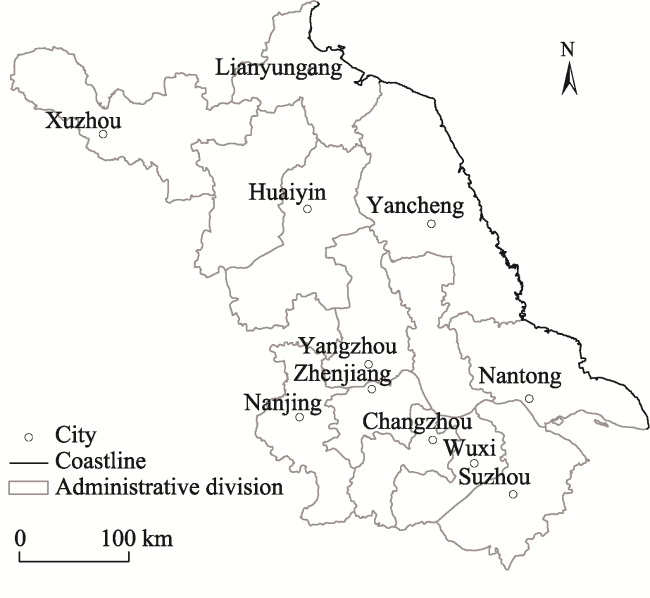
Fig. 1 Location of Jiangsu Province, China |
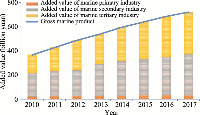
Fig. 2 Added value of the three types of marine industries in Jiangsu Province |
Table 1 Evaluation standard of marine sustainable development |
| Grade | Ⅴ | Ⅳ | Ⅲ | Ⅱ | Ⅰ |
|---|---|---|---|---|---|
| Evaluation indicator value | [0, 0.2) | [0.2, 0.4) | [0.4, 0.6) | [0.6, 0.8) | [0.8, 1.0] |
| State | Very bad | Bad | Neutral | Good | Very good |
Table 2 Evaluation indicator system of marine sustainable development |
| System layer | Indicator layer | Unit | Coefficient of variation weight |
|---|---|---|---|
| Marine economy | Added value of marine industry (X1) | ×108 yuan | 0.0460 |
| Gross marine product of coastal areas (X2) | ×108 yuan | 0.0488 | |
| The proportion of marine GDP to coastal GDP (X3) | % | 0.0120 | |
| Proportion of marine secondary industry in marine GDP in coastal areas (X4) | % | 0.0074 | |
| Proportion of marine tertiary industry in marine GDP in coastal areas (X5) | % | 0.0083 | |
| Number of employed personnel involved in the sea (X6) | ×104 person | 0.0138 | |
| Passenger traffic volume in coastal areas (X7) | ×104 person | 0.0770 | |
| Marine resources | Cargo throughput of coastal ports (X8) | ×104 t | 0.0419 |
| Per capita water resources in coastal areas (X9) | m3 person-1 | 0.0273 | |
| Mariculture area in coastal area (X10) | ×104 ha | 0.0093 | |
| Coastal wind power generation capacity (X11) | ×104 kW | 0.0758 | |
| Coastal wetland area (X12) | ×104 ha | 0.0288 | |
| Area of marine nature reserves in coastal areas (X13) | ×104 ha | 0.1950 | |
| Marine biodiversity (X14) | 0.0548 | ||
| Marine environment | Economic losses caused by storm surges in coastal areas (X15) | ×108 yuan | 0.2351 |
| Industrial wastewater discharge in coastal areas (X16) | ×104 t | 0.0110 | |
| Standard rate of industrial wastewater discharge in coastal areas (X17) | % | 0.0011 | |
| Industrial waste gas emissions in coastal areas (X18) | ×108 m3 | 0.0242 | |
| Industrial smoke (dust) emission in coastal areas (X19) | ×108 m3 | 0.0073 | |
| Disposal capacity of industrial solid waste in coastal areas (X20) | ×104 t | 0.0583 | |
| Comprehensive utilization of industrial solid waste in coastal areas (X21) | ×104 t | 0.0165 |
Table 3 Marine sustainable development based on the grey relational model |
| Year | Grey relational degree of correlation coefficient average method | Grey relational degree of weighting method | Average value of grey relational degree | Rank |
|---|---|---|---|---|
| 2016 | 0.7146 | 0.5881 | 0.6513 | 1 |
| 2012 | 0.5782 | 0.6246 | 0.6014 | 2 |
| 2014 | 0.6345 | 0.5259 | 0.5802 | 3 |
| 2015 | 0.6273 | 0.521 | 0.5741 | 4 |
| 2013 | 0.6097 | 0.5382 | 0.5739 | 5 |
| 2011 | 0.5383 | 0.4455 | 0.4919 | 6 |
| 2010 | 0.5487 | 0.4323 | 0.4905 | 7 |
| 2008 | 0.4590 | 0.4941 | 0.4766 | 8 |
| 2009 | 0.4571 | 0.3834 | 0.4203 | 9 |
| 2006 | 0.4474 | 0.3634 | 0.4054 | 10 |
| 2007 | 0.4069 | 0.3632 | 0.3850 | 11 |
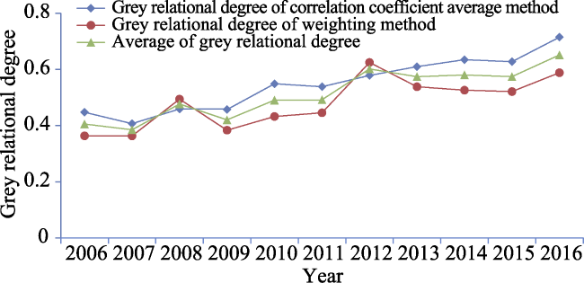
Fig. 3 Comparison of dynamic trends of the evolution of marine sustainable development based on the average correlation coefficient method and the weighting method |
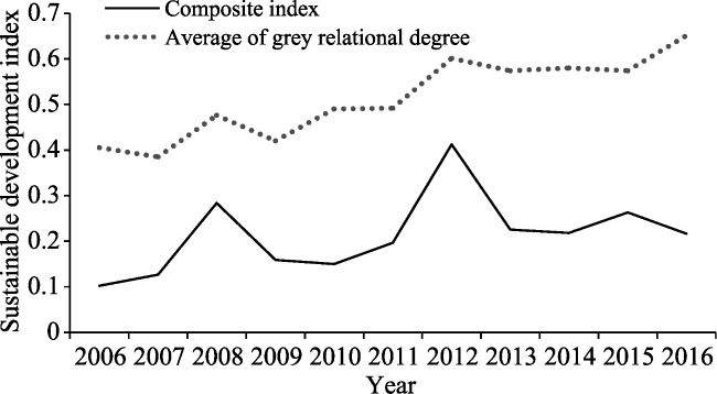
Fig. 4 Comparison of dynamic trend of the evolution of marine sustainable development based on the grey relational model and the comprehensive index model |
Table 4 Output results of normality test |
| Dependent variable (Y) | Kolmogorov- Smirnov(a) | Shapiro-Wilk | ||||
|---|---|---|---|---|---|---|
| Statistic | df | Sig. | Statistic | df | Sig. | |
| Average value of grey relational degree of marine sustainable development | 0.190 | 3 | 0.998 | 3 | 0.905 | |
Table 5 Model overview output |
| R | R2 | Adjusted R2 | Std. Error of the estimate |
|---|---|---|---|
| 0.951a | 0.905 | 0.894 | 0.0287146 |
Note: Predictive variable (X8). |
Table 6 Decomposition of simple correlation coefficients |
| Driving factors | The correlation coefficient of Y | Direct path coefficient | Indirect path coefficient total |
|---|---|---|---|
| X8 | 0.951 | 0.951 | 0 |
Table 7 Main driving factors of marine sustainable development |
| Indicator | Grey relational degree of correlation coefficient average method | Grey relational degree of weighting method | Average value of grey relational degree | Driving force ranking |
|---|---|---|---|---|
| X15 | 0.0351 | 0.1975 | 0.1163 | 1 |
| X13 | 0.0357 | 0.1666 | 0.1012 | 2 |
| X11 | 0.0454 | 0.0824 | 0.0639 | 3 |
| X14 | 0.0519 | 0.0681 | 0.0600 | 4 |
| X7 | 0.0405 | 0.0746 | 0.0575 | 5 |
| X2 | 0.0498 | 0.0583 | 0.0540 | 6 |
| X1 | 0.0475 | 0.0524 | 0.0500 | 7 |
| X20 | 0.0410 | 0.0572 | 0.0491 | 8 |
| X8 | 0.0473 | 0.0474 | 0.0474 | 9 |
| X6 | 0.0659 | 0.0218 | 0.0438 | 10 |
| X3 | 0.0673 | 0.0193 | 0.0433 | 11 |
| X12 | 0.0501 | 0.0346 | 0.0423 | 12 |
| X21 | 0.0525 | 0.0207 | 0.0366 | 13 |
| X9 | 0.0426 | 0.0279 | 0.0353 | 14 |
| X10 | 0.0564 | 0.0126 | 0.0345 | 15 |
| X4 | 0.0536 | 0.0095 | 0.0316 | 16 |
| X17 | 0.0583 | 0.0016 | 0.0299 | 17 |
| X16 | 0.0464 | 0.0123 | 0.0293 | 18 |
| X18 | 0.0352 | 0.0205 | 0.0279 | 19 |
| X5 | 0.0415 | 0.0083 | 0.0249 | 20 |
| X19 | 0.0360 | 0.0063 | 0.0212 | 21 |
| 1 |
|
| 2 |
|
| 3 |
|
| 4 |
|
| 5 |
|
| 6 |
|
| 7 |
|
| 8 |
|
| 9 |
|
| 10 |
|
| 11 |
|
| 12 |
|
| 13 |
|
| 14 |
|
| 15 |
|
| 16 |
|
| 17 |
|
| 18 |
|
| 19 |
|
| 20 |
|
| 21 |
|
| 22 |
|
| 23 |
|
| 24 |
|
/
| 〈 |
|
〉 |