
Journal of Resources and Ecology >
Forecasting Gas Consumption Based on a Residual Auto-Regression Model and Kalman Filtering Algorithm
Received date: 2018-09-19
Accepted date: 2019-06-05
Online published: 2019-10-11
Supported by
Foundation: Soft Science Research Project in Shanxi Province of China(2017041030-5)
Science Fund Projects in North University of China (XJJ2016037).()
Copyright
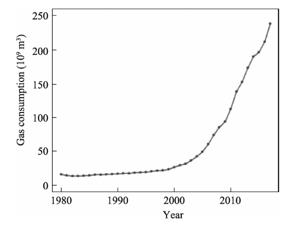
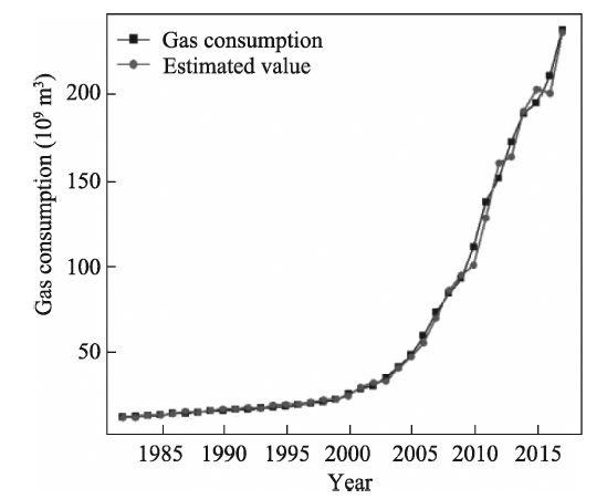
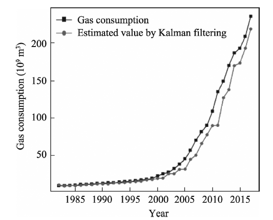
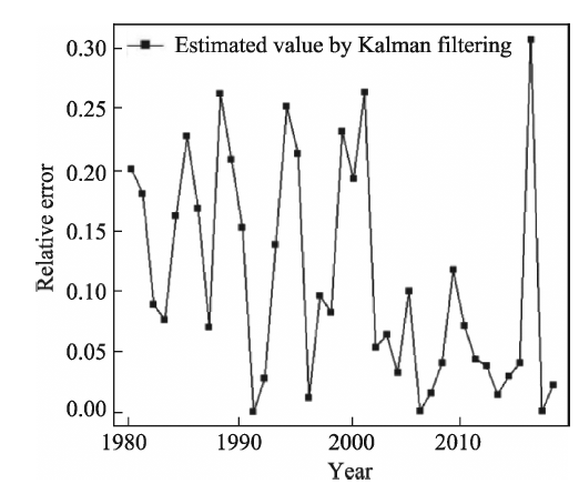
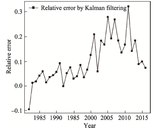
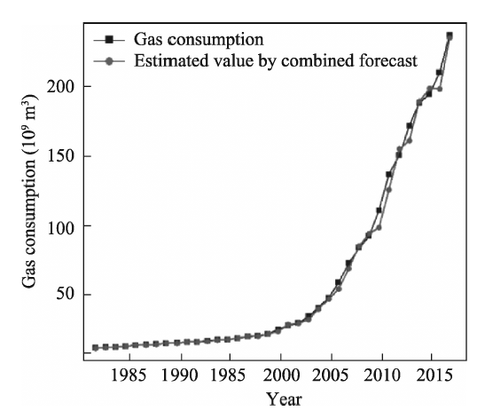
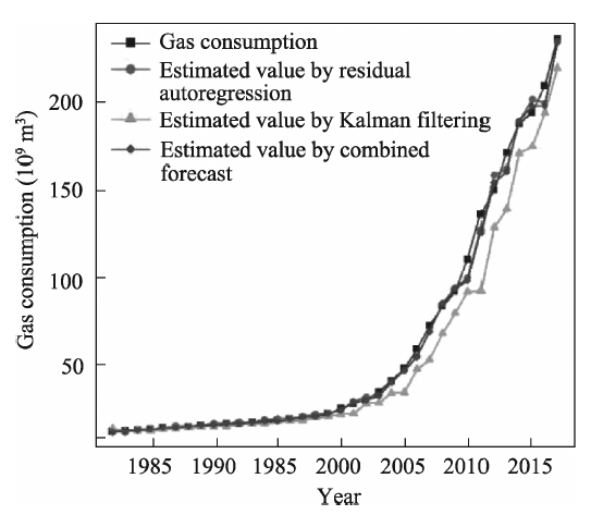
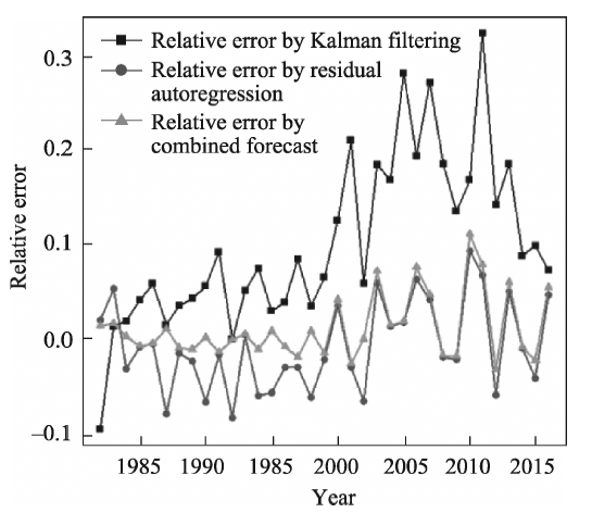
Consumption of clean energy has been increasing in China. Forecasting gas consumption is important to adjusting the energy consumption structure in the future. Based on historical data of gas consumption from 1980 to 2017, this paper presents a weight method of the inverse deviation of fitted value, and a combined forecast based on a residual auto-regression model and Kalman filtering algorithm is used to forecast gas consumption. Our results show that: (1) The combination forecast is of higher precision: the relative errors of the residual auto-regressive model, the Kalman filtering algorithm and the combination model are within the range (-0.08, 0.09), (-0.09, 0.32) and (-0.03, 0.11), respectively. (2) The combination forecast is of greater stability: the variance of relative error of the residual auto-regressive model, the Kalman filtering algorithm and the combination model are 0.002, 0.007 and 0.001, respectively. (3) Provided that other conditions are invariant, the predicted value of gas consumption in 2018 is 241.81×10 9 m 3. Compared to other time-series forecasting methods, this combined model is less restrictive, performs well and the result is more credible.
ZHU Meifeng , WU Qinglong , WANG Yongqin . Forecasting Gas Consumption Based on a Residual Auto-Regression Model and Kalman Filtering Algorithm[J]. Journal of Resources and Ecology, 2019 , 10(5) : 546 -552 . DOI: 10.5814/j.issn.1674-764X.2019.05.011
Table 1 Observated values and the fitting values of each prediction method (unit: 109 m3) |
| Year | Observed value | Estimated value of residual auto-regression | Estimated value of Kalman | Estimated value of combined forecast | Year | Observed value | Estimated value of residual auto-regression | Estimated value of Kalman | Estimated value of combined forecast |
|---|---|---|---|---|---|---|---|---|---|
| 1982 | 12.33 | 12.06 | 13.48 | 12.13 | 2000 | 25.35 | 24.43 | 22.13 | 24.25 |
| 1983 | 12.61 | 11.92 | 12.42 | 12.39 | 2001 | 28.37 | 29.17 | 22.39 | 29.05 |
| 1984 | 12.84 | 13.22 | 12.58 | 12.79 | 2002 | 30.19 | 32.12 | 28.36 | 30.14 |
| 1985 | 13.36 | 13.45 | 12.79 | 13.43 | 2003 | 35.08 | 32.93 | 28.58 | 32.51 |
| 1986 | 14.22 | 14.26 | 13.36 | 14.26 | 2004 | 41.04 | 40.43 | 34.06 | 40.38 |
| 1987 | 14.35 | 15.45 | 14.11 | 14.17 | 2005 | 48.21 | 47.29 | 34.62 | 47.23 |
| 1988 | 14.84 | 15.03 | 14.29 | 14.95 | 2006 | 59.31 | 55.47 | 47.76 | 54.70 |
| 1989 | 15.53 | 15.86 | 14.84 | 15.67 | 2007 | 72.95 | 69.81 | 53.10 | 69.40 |
| 1990 | 15.76 | 16.77 | 14.85 | 15.70 | 2008 | 84.09 | 85.52 | 68.39 | 85.38 |
| 1991 | 16.42 | 16.66 | 14.88 | 16.62 | 2009 | 92.60 | 94.45 | 79.96 | 94.15 |
| 1992 | 16.41 | 17.74 | 16.39 | 16.39 | 2010 | 111.18 | 100.68 | 92.35 | 98.70 |
| 1993 | 17.32 | 17.21 | 16.40 | 17.20 | 2011 | 137.08 | 127.64 | 92.63 | 126.13 |
| 1994 | 17.92 | 18.95 | 16.55 | 18.08 | 2012 | 150.94 | 159.51 | 129.35 | 155.41 |
| 1995 | 18.33 | 19.33 | 17.76 | 18.14 | 2013 | 171.92 | 163.04 | 139.83 | 161.39 |
| 1996 | 19.10 | 19.64 | 18.32 | 19.22 | 2014 | 188.40 | 189.86 | 171.53 | 189.72 |
| 1997 | 20.19 | 20.76 | 18.45 | 20.54 | 2015 | 194.76 | 202.38 | 175.21 | 200.80 |
| 1998 | 20.93 | 22.17 | 20.17 | 20.72 | 2016 | 210.34 | 200.11 | 194.72 | 211.50 |
| 1999 | 22.21 | 22.65 | 20.72 | 22.49 | 2017 | 237.30 | 235.40 | 220.27 | 235.21 |
| [1] |
|
| [2] |
|
| [3] |
|
| [4] |
|
| [5] |
|
| [6] |
|
| [7] |
|
| [8] |
|
| [9] |
|
| [10] |
|
| [11] |
|
| [12] |
|
| [13] |
|
| [14] |
|
/
| 〈 |
|
〉 |