Plant Ecosystem

Species Abundance Distribution Patterns of a Toona ciliata Community in Xingdoushan Nature Reserve

  • WANG Yang 1 ,
  • ZHU Shengjie 2 ,
  • LI Jie 2 ,
  • HE Xiuling 2 ,
  • JIANG Xiongbo , 1, * ,
  • ZHANG Min , 1, *
Expand
  • 1.Hubei Ecology Polytechnic College, Wuhan 430200, China
  • 2.Guangdong Polytechnic of Environmental Protection Engineering, Foshan, Guangdong 528216, China
* JIANG Xiongbo, E-mail:
ZHANG Min, E-mail:

Received date: 2019-03-11

  Accepted date: 2019-05-31

  Online published: 2019-10-11

Supported by

Public Welfare Research Project of Department of Science and Technology in Hubei Province(40 2012DBA40001)

Scientific Research Project of Department of Education in Hubei Province(B20160555)

Copyright

Copyright reserved © 2019

Abstract

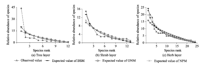
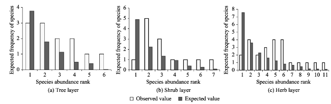
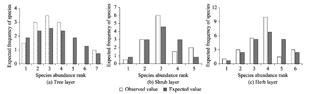
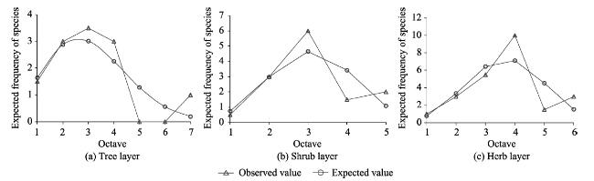
With the goal of model fitting species abundance distribution patterns of the tree, shrub and herb layers of the natural Toona ciliata community in Xingdoushan Nature Reserve, Enshi Autonomous Prefecture, Hubei Province, we used the data collected from the field survey and employed different ecological niche models. The models tested were the broken stick model (BSM), the overlapping niche model (ONM) and the niche preemption model (NPM), as well as three statistic models, the log-series distribution model (LSD), the log-normal distribution model (LND) and the Weibull distribution model (WDM). To determine the fitted model most suitable to each layer, the fitting effects were judged by criteria of the lowest value of Akaike Information Criterion (AIC), Chi-square and the K-S values with no significant difference (P>0.05) between the theoretical predictions and observed species abundance distribution values. The result showed: (1) The fitting suitability and goodness of fit of the tree, shrub and herb layers by using the three ecological niche models were ranked as: NPM>BSM>ONM. Of the three statistical models, by accepting the fitting results of the three layers, WDM was the best fitting model, followed by LND. By rejecting the fitting tests of the herb layer, LSD had the worst fitting effect. The goodness of the statistical models was ranked as: WDM>LND>LSD. In general, the statistical models had better fitting results than the ecological models. (2) T. ciliata was the dominant species of the tree layer. The species richness and diversity of the herb layer were much higher than those of either the tree layer or the shrub layer. The species richness and diversity of the shrub layer were slightly higher than those of the tree layer. The community evenness accorded to the following order: herb>shrub>tree. Considering the fitting results of the different layers, different ecological niche models or statistical models with optimal goodness of fit and ecological significance can be given priority to in studying the species abundance distribution patterns of T. ciliata communities.

Cite this article

WANG Yang , ZHU Shengjie , LI Jie , HE Xiuling , JIANG Xiongbo , ZHANG Min . Species Abundance Distribution Patterns of a Toona ciliata Community in Xingdoushan Nature Reserve[J]. Journal of Resources and Ecology, 2019 , 10(5) : 494 -503 . DOI: 10.5814/j.issn.1674-764X.2019.05.004

1 Introduction

The study of species abundance distribution patterns is one of the main approaches for the quantitative study of community structure and an important foundation for understanding community features. The distribution of species diversity can reflect the arrangement and species patterns on certain spatial and temporal scales, which can be used to
explore the possible ecological processes that may be unforeseen in the community construction, so we can further understand the formation and mechanisms of species diversity maintenance in the ecosystem (Borda de Águ et al., 2012).
Since the 1930s, the study of species abundance distribution patterns has become an important approach for revealing the community organizational structure and the regional species distribution laws (Ma, 2003). Researchers have tentatively applied various statistical models to the study of species abundance distribution patterns. The log-series distribution model (Fisher et al., 1943), the log-normal distribution model (Preston, 1948), the negative binomial distribution model (Kempton, 1979; Ma et al., 1997) and the Weibull distribution model (Qin et al., 2009; Wu et al., 1997) have been used to explore the mechanism of species abundance distribution patterns. With the ecological mechanism as a priority, models focusing on the ecological mechanism, such as the overlapping niche model, the niche preemption model (Whittaker, 1972; Pielou, 1975) and the neutral theory model (Hubbell, 2001), have been widely used in the study of species abundance distribution patterns.
With the continuing development of ecological and computer sciences, researchers have successively integrated ecological theory into mathematical statistics, and gradually established research models for species abundance distribution patterns that have ecological significance (Tokeshi, 1993). The parameters of the applied distribution models or the shapes of distribution curves can be used as measurement indexes for community research and can reflect the dynamics of community diversities, which cannot be achieved by any conventional species diversity indexes (Magurran, 1988). Species abundance distribution models, therefore, are more effective than mere diversity indexes in the recognition of a community (Tokeshi, 1993).
Toona ciliata Roem., also known as Honglianzhi (a local name), is a deciduous or semi-evergreen tall tree, and a precious timber species belonging to genus Toona, Meliaceae, which was listed as a wild endangered species under secondary national protection (The State Council of the People’s Republic of China, 1999). Excessive human exploits and slow natural regeneration of T. ciliata has resulted in the decrease of its natural distribution areas, the fragmentation of its habitats, and the reduction of plant individuals in number. The study of species abundance distribution patterns will provide ecological bases for species protection, and bear great significance in biodiversity management (Tokeshi, 1993).
Three ecological niche models, namely the broken stick model (BSM), the niche preemption model (NPM), and the overlapping niche model (ONM), and three statistical models, the log-series distribution model (LSD), the log-normal distribution model (LND) and the Weibull distribution model of density function (WDM), were used to fit the species abundance distribution patterns of the tree, shrub and herb layers in the T. ciliata community of Xingdoushan Nature Reserve. The fitting results obtained were verified with the Kolmogorov Smirnov (K-S) test, the chi-square (χ2) test and the AIC criterion (Akaike information criterion). The overall purpose of this research was to explore the species compositions and abundance distribution regularities of different vegetation layers in the community dominated by T. ciliata, and to provide a scientific reference for illuminating the T. ciliata community structure of Xingdoushan Nature Reserve.

2 Materials and methods

2.1 Study area

The research area (29°57ʹ-30°10ʹN, 108°57ʹ-109°27ʹE, elevation 716-722 m) is located in Xingdoushan National Nature Reserve in Enshi Prefecture, Hubei Province. The Nature Reserve falls in the transitional zone between the central subtropical zone and the north subtropical zone, in which the subtropical continental monsoon climate is characterized by warm and humid conditions and even rainfalls. The high mountains on all sides surround the Nature Reserve, forming a long, closed valley that serves as a “sanctuary” for plants (Huang et al., 2016). Its geomorphic transitional nature makes research of the Xingdoushan National Nature Reserve of high scientific value and practical significance for vegetation geography, flora geography and biodiversity conservation (Huang et al., 2016). Within the area, the annual average temperature is about 14.9℃, the frost-free period is about 210 d, the average rainfall is about 1471.7 mm, and the average relative humidity is about 81.6%. The loose mountain yellow soil was developed from argillaceous shale, which is mainly composed of flat sandy soil. With abundant hydrothermal resources and undulating mountains, luxurious vegetation exists (Liu et al., 2007; Chen et al., 2008; Huang et al., 2016). The main vegetation types are evergreen broad-leaved forest, mixed evergreen and deciduous broad-leaved forest.
The research site is on the lower slope on a gradient of about 31°, with an aspect of southwest 40°. T. ciliata was the dominant species in the over-mature forest, with a canopy density of 0.77. The main arbor species in the research community included T. ciliata, Litsea hupehana, Rhus punjabensis, and Styrax suberifolius. Common shrub species included Paragutzlaffia henryi, Rubus malifolius and Clerodendrum bungee. The main herbaceous species included Elatostema umbellatum, Paragutzlaffia henryi, Selaginella remotifolia and Fagopyrum dibotrys.

2.2 Research methods

The survey was conducted in 2015. According to the habitat situation, one sample plot was set up, covering all surviving T. ciliata plants, with 20 m × 20 m in area. Sixteen sample quadrates were set within each plot, and each was 5 m × 5 m in size. At the four corners and the center of the sample plot, five shrub quadrates were set, each 5 m × 5 m in size, and five herb quadrates with 1 m × 1 m areas were established. All plants in the plots were investigated in detail, and the names, the number of plants (clusters), coverage, height, species frequency, growth status and distribution status were recorded. Ground diameters and heights of plants with diameters at breast height (DBH) less than 2.5 cm were measured. For living plants with DBH larger than 2.5 cm, DBH, crown width and the first subbranch height were recorded. The species number was determined and counted.

2.3 Fitting models

2.3.1 Ecological niche models
The broken stick model (BSM) is a hypothesis model for random ecological niches proposed by MacArthur (1957). BSM is a resource-allocation model, in which the random allocation of species abundance is along a one-dimensional gradient (MacArthur, 1957; Cheng et al., 2011). Suppose that the species number in a community is S, and the total species abundance is equal to 1, arranged along a stick. S-1 points are randomly set along the stick, which divide the stick into S parts. The lengths of individual parts represent the degrees of various species abundances. Random segments from the longest to the shortest are arranged to be equivalent to the species arrangement from the most common to the rarest. The abundance ni of the ith species can be expressed as:
${{n}_{i}}=\frac{N}{S}\underset{x=i}{\overset{S}{\mathop \sum }}\,\frac{1}{x}$
where S is the species number and N represents the total number of species in the community (and they have the same meanings hereafter).
The niche preemption model (NPM), also known as the geometric progression model, assumes that there are S species and N plants in a community and the limited resources are equal to 1. The first species with maximum abundance occupies k part of the total niche ratio of the community. The second species takes up the remaining, that is k × (1-k), part of the total, and the third species covers the leftover resources, that is the k × (1-k)2 part, and so forth (Whittaker, 1972; Qin et al., 2009). Therefore, the species number along the stick that is taken up by the ith species abundance is:
${{n}_{i}}=N\frac{k{{(1-k)}^{i-1}}}{1-{{(1-k)}^{S}}}\ \ \ \ (i=1,2,3\cdots )$
The undetermined parameter value ranges between 0 and 1, and the smaller the value of k, the more species a community has. A higher k value indicates more significant dominance of the dominant species in the community, and less evenness of the community. The k value can be solved through the following formula with iteration:
$\frac{~{{n}_{\text{min}}}}{N}=\text{ }\!\!~\!\!\text{ }\frac{k{{(1-k)}^{S-1}}}{1-{{(1-k)}^{S}}}$
where nmin is the species number of the lowest species abundance value in the community.
Overlapping niche model (ONM). The whole niche of a community is still regarded as a stick in the ONM, each species abundance is equal to the distance between two random points along the stick, and each species is independent of the others. As each species takes up niche resources along the stick as needed, there are unavoidable overlaps in occupying resources between species, and, therefore, the whole niche or total resources of the community is no longer 1 (MacArthur, 1957). The proportional Pi corresponding to the theoretical abundance is:
${{P}_{i}}=1-\frac{2i}{2i+1}(1-{{P}_{i+1}})\ \ \ \ (i=S-1,S-2,S-3,\cdots )$
where Pi indicates the proportion in accordance with the theoretical abundance.
2.3.2 Statistical models
Log-series distribution model (LSD). LSD is suitable for describing positive integers excluding 0, that is, species without actual existence are not considered. This model predicts the frequency of species with r individuals (Fisher et al., 1943; Ma et al., 1997):
$\text{ }\!\!~\!\!\text{ }{{f}_{r}}=\frac{\alpha {{x}^{r}}}{r}\ \ \ \ (r=\text{ }1,2,3,4,\cdots )$
In LSD, α represents the characteristic of a community. It can be used as a diversity index and its value is greater than 0. x is a constant (0 < x ≤ 1) that is related to the size of the sample plot (Pielou, 1975). x can be iteratively solved firstly, and then α can be calculated with the following formula:
$\frac{S}{N}=\frac{1-x}{x}[-\text{ln}(1-x)];\begin{matrix} {} \\ \end{matrix}x=\frac{N}{\alpha +N}$
Log-normal distribution model (LND). LND refers to the log-normal distribution truncated at the left end, rather than the complete log-normal distribution, and was introduced by Preston (1948). In the order of community species abundance from the smallest to the largest, the octave method was used to group observed frequencies of species abundances (Preston, 1948; Qin et al., 2009). The formula of logarithmic normal distribution is expressed as follows:
${{S}_{(R)}}={{S}_{0}}\text{exp}(-{{\lambda }^{2}}{{R}^{2}})$
S(R) is the species number in the Rth octave, R means the number of the octaves, and S0 represents the species number of the octave with the greatest number of species. λ is the reciprocal of the width of normal distribution curves, which is a parameter related to sample size. Higher values of λ indicate a thinner and higher curve, and there will be a higher species density in the community. Conversely, a smaller λ indicates a more discrete species distribution in the community (Gao et al., 2011).
The Weibull distribution model of density function (WDM) is given by:
$f(x)=\frac{c}{b}{{\left( \frac{x-a}{b} \right)}^{c-1}}\times {{\text{e}}^{\left[ -{{\left( \frac{x-a}{b} \right)}^{c}} \right]}}\ \ (a\ge 0,b>0,c>0) $
where f(x) is the simulated frequency of a species to x degree, with three relevant parameters: a, the position parameter; b, the scale parameter; and c, the curve shape parameter. c can more precisely reflect a distribution curve. When c < 1, the curve presents an inverted J-shaped distribution; when 1 < c < 3.6, the curve demonstrates a positive mountain-like distribution; when c = 3.6, the curve is an approximately normal distribution; and when c > 3.6, the curve exhibits a negative mountain-like distribution (Wu and Hong, 1997; Qin et al., 2009). Since the minimum species abundance can be treated as 0, and so can the parameter a, then the model with 2 parameters (b and c) is adopted. The maximum likelihood method is employed to solve the two parameters b and c (Qin, 2009; Qin et al., 2009).

2.4 Fitting test for models

With species numbers as the abundance index, the Kolmogorov-Smirnov (K-S) and chi-square (χ2) tests were used to verify the fitting results of the above six models. The P value of testing significance was set at two levels (0.01 and 0.05) to determine an optimal model for each layer. Data processing, statistics and model fitting were completed using Excel 2007, and testing was completed using the R language.
AIC information criterion. In 1974, Japanese scholar Akaike put forward AIC, based on the principle of maximum likelihood estimation (Burnham and Anderson, 2002). AIC is a standard for measuring the goodness of fit of models. Based on the concept of information entropy, the complexity and goodness of fit of an estimated model can be weighed by the following formula:
AIC = 2ln(L) + 2K
where K is the number of parameters and L is the maximum likelihood function. AIC is applied to the selection of regression models. It is assumed that the random error of a regression model is an independent normal distribution. The AIC formula of the regression model can be as follows:
AIC = 2K + n ln(RSS/n)
where n represents the sample size and RRS is the sum of squared residuals. AIC provides a standard for weighing model complexity and the model’s ability to optimally describe data, and it seeks an equilibrium between the above- mentioned complexity and the model’s descriptive ability. The model with the AIC minimum contains the fewest free parameters, and the data can be best interpreted by the model with the AIC minimum. The R language was used to calculate AIC values.

3 Results and analysis

3.1 Ecological models

Three ecological models, the broken stick model (BSM), the overlapping niche model (ONM) and the niche preemption model (NPM), were used to fit the species abundance of the tree, shrub and herb layers in the T. ciliata community. AIC values were used to select the optimal models, but a model could not be rejected through AIC value alone (Gao et al., 2011). The fitted model was selected with a relatively lower AIC value, a lower χ2 and a lower K-S value (P>0.01, P>0.05) as three distinct selection principles.
Table 1 shows the fitting tests of the tree, shrub, and herb layers in the T. ciliata community with BSM, ONM and NPM. The χ2 test rejected BSM fitting of the tree layer (P<0.01). The shrub layer (AIC=2.461, P of χ2 0.837, P of K-S test 0.570) and the herb layer (AIC=21.342, P of χ2 0.991 and P of K-S test 0.893) were both suitable for BSM fitting, and the fitting effect of the herb layer was better than that of the shrub layer.
Table 1 Fitting test results of various ecological niche models
Model Tree layer Shrub layer Herb layer
AIC value χ2 test K-S test AIC value χ2 test K-S test AIC value χ2 test K-S test
χ2 P value D P value χ2 P value D P value χ2 P value D P value
BSM 30.679 39.461 0* 0.333 0.518 2.461 6.516 0.837 0.308 0.570 21.342 9.426 0.991 0.167 0.893
ONM 29.911 73.339 0* 0.417 0.249 10.258 7.820 0.729 0.308 0.570 31.309 13.637 0.914 0.208 0.675
NPM 33.077 43.877 0* 0.250 0.847 5.713 4.245 0.962 0.231 0.879 27.675 7.405 0.998 0.167 0.893

P<0.01.

The testing results revealed that ONM could not explain the species abundance distribution of the tree layer, but could accept those of the shrub layer (AIC=10.258, P of χ2 0.837, P of K-S test 0.570) and the herb layer (AIC=31.309, P of χ2 0.914, P of K-S test 0.675), and, comparatively, ONM had the best fitting effect on the herb layer.
The k value of NPM is usually related to the number of species in a community. The smaller the k value is, the larger the number of species in a community (Qin, 2009). The larger the k value is, the more obvious is the degree of abundance of the dominant species, and the smaller the evenness of the community (Gao et al., 2011). k values in the three vegetation layers were 0.235, 0.179 and 0.122, respectively, which were contrary to the species numbers investigated. The testing results showed that NPM also rejected the tree layer, with P of the χ2 test 0, showing that the difference was very significant. But in the shrub layer (AIC=5.713, P of χ2 0.962, P of K-S test 0.879) and the herb layer (AIC=27.675, P of χ2 0.998, P of K-S test 0.893), the NPM fitting effects were optimal.
With the species number as the abscissa and the relative species abundance as the ordinate, the curves of the three ecological niche models for the three layers in the T. ciliata community are shown in Fig. 1. The abscissa directly reflects the species richness, the sizes of which were: herb>shrub>tree; the steepness of the curves in the vertical coordinate could directly reflect the evenness changes of the various vegetation layers (Guo et al., 2007). The evenness of the herb layer was the highest, while that of the shrub layer was in the middle and that of the tree layer was the lowest. The relative species abundances of the three layers were: herb>tree>shrub; and the relative abundances of only a few species in the tree layer were larger, so the evenness was lower. The distributions of most species in the shrub layer and the herb layer were more even.

Fig. 1 Fitted curves of the ecological niche distribution models

It can also be seen from Fig. 1 that species abundance of the tree layer did not conform to the distribution fittings with BSM, ONM or NPM, and the fitted curves deviated from the observed ones. However, BSM, ONM and NPM could explain the fittings of shrubs and herbs in the community. The distribution curves of the observed values were close to those of the predicted values. As can be seen from Fig. 1, the best fitting result of the shrub layer was with NPM, followed by BSM and ONM. The optimal fitting model of the herbaceous layer was NPM, followed by BSM and ONM in order.
Because the abundance of T. ciliata was very significant, there were larger individual differences among species in the tree layer. The dominant species in the community were very competitive and occupied a large part of the ecological niche, so the fitting effect of the ecological niche model was undesirable. Since the niche models of species abundance emphasize resource allocation among species, the species abundances of the shrub layer and the herb layer were relatively similar, and each species could take the required resources to coexist harmoniously according to its own needs. Therefore, BSM, ONM and NPM had better fitting effects on the shrub and herb layers in the community.

3.2 Analyses of statistical models

3.2.1 LSD and LND model fitting and testing
The fitting parameters of the tree, shrub and herb layers with LSD, LND and WDM in the T. ciliata community of Xingdoushan Nature Reserve are shown in Table 2. LSD parameter α represents species diversity (Magurran and Henderson, 2003), reflects the characteristics of different forest layers and shows the diversity differences among communities. As can be seen in Table 2, α values of the three layers were 3.959, 5.374 and 7.952, respectively. When the value of α is lower, the number of clustered species is higher than that of rare species, indicating that high diversity is positive for the conservation of rare species (Reng et al., 2009).
Table 2 Parameters of LSD and LND and the fitting test results
Vegetation
layer
LSD LND
x value α value AIC value χ2 test K-S test S0 value λ value AIC value χ2 test K-S test
χ2 P value D P value χ2 P value D P value
Tree layer 0.952 3.959 -0.469 0.999 0.318 0.500 0.441 2.566 0.280 -8.530 3.989 0.408 0.429 0.541
Shrub layer 0.911 5.374 8.268 6.757 0.009** 0.203 0.571 4.573 0.656 1.802 3.010 0.222 0.200 1.000
Herb layer 0.951 7.952 18.469 6.978 0.031* 0.545 0.076 6.766 0.506 8.077 4.648 0.200 0.167 1.000

**P<0.01, *P<0.05.

In the LND fitting process, the octave numbers of the tree, shrub and herbaceous layers were 7, 5 and 6, and the individual species numbers were differentiated in different octaves. S0 stands for the group with the maximum species in the model octave, and the values of S0 were 2.566, 4.753 and 6.766, respectively, in the different forest layers. From the change of λ values, λ was 0.280 (tree), 0.656 (shrub) and 0.506(herb), indicating that the community species distribution tended to be concentrated. The change of the S0 value might be consistent with the size of species diversity, but the trend of species distribution concentration might not necessarily be affected by the size of diversity.
In the data from Table 2, the fitting results of AIC, the χ2 test and the K-S test all showed that LSD accepted the fitting models of the tree layer (AIC= -0.469, P of χ2 and P of K-S test 0.318 and 0.441, respectively), but rejected the fitting of the shrub layer (P<0.01) and the herbaceous layer (P<0.05). LND could accept the species abundance distribution fitting of the tree, shrub and herb layers of the T. ciliata community (P>0.05), with the widest fitting suitability and better fitting effect. In comparison, the shrub layer had the best fitting effect, followed by the herb layer and the tree layer.
3.2.2 WDM fitting and testing
Octave grouping was also adopted in the course of WDM fitting (Preston, 1948; Qin et al., 2009), and the octave was the same as that in LND. Since the minimum species abundance can be treated as 0, the parameter a can also be 0, making the model into a two-parameter Weibull model (Preston, 1948; Qin, 2009). Parameter b does not fully reflect the size of the octave grouping (Zhang et al., 2018), because b may be restricted by the sampling area (Qin et al., 2009). Shape parameter c can be used as an indicator with certain ecological significance to reflect the features of community species diversity (Wu et al., 2004), and it can better reflect the shapes of fitted curves. From Table 3, we can determine that the parameter c of the three layers was: 1 < c < 3.6, showing that the curves presented positive mountain-like distributions. The values of average evenness E of the tree, shrub and herb were 0.658, 0.879 and 0.898, respectively. The c value was generally close to 3.6, meaning it was closer to a normal distribution. Table 3 also shows that the species abundance distribution of the tree layer was uneven, and the species composition was dominated by a few species, which was almost the same as the data in the actual survey. The numbers of most species in the shrub layer and the herb layer increased gradually, so did the diversity index and evenness (Shannon-Weiner index of the tree, shrub and herb layers were 1.634, 2.255 and 2.855, respectively). The WDM fitting test showed that WDM could better fit the species abundance distribution pattern of the tree layer, and optimally fit the shrub and the herb layers (P>0.05) of the T. ciliata community.
Table 3 Parameters of WDM and the fitting test results
Vegetation layer a value b value c value WDM AIC value χ2 test K-S test
χ2 P value D P value
Tree layer 0 3.492 2.146 $f(x)=0.147{{x}^{1.146}}{{e}^{\frac{-{{x}^{2.146}}}{14.636}}}$ -5.516 5.598 0.133 0.286 0.938
Shrub layer 0 3.480 3.213 $f(x)=0.059{{x}^{2.213}}{{e}^{\frac{-{{x}^{3.213}}}{54.9401}}}$ 2.723 2.322 0.128 0.200 1.000
Herb layer 0 4.136 3.241 $f(x)=0.033{{x}^{2.241}}{{e}^{\frac{-{{x}^{3.241}}}{99.626}}}$ 8.254 4.832 0.089 0.333 0.893
3.2.3 Correlation analyses of fitted parameters and diversity
According to the correlation analyses of species richness, the Shannon-Weiner index H and Pielou evenness E in the tree, shrub and herbaceous layers with the parameters of different statistical models (Table 4), the LSD parameter x had a low correlation with H and E. α was highly correlated with species richness S (r=0.961), H (r=0.984) and E (r=0.888), indicating that α was an effective indicator of community diversity in the LSD fitting (Magurran, 1988; McGill, 2010). λ of LND had higher correlations with H (r=0.605) and E (r=0.888), showing that the tendency of the concentration of species abundance distribution expressed by λ was consistent with the species diversity indexes. The scale parameter b of WSM was highly correlated with H (r=0.853) and E (r=0.547). The c value was correlated with H (r=0.882) and significantly correlated with E (r=0.999), revealing that the c value had obvious ecological significance (Wu et al., 2004) and could explain species diversity indexes.
Table 4 Correlation analysis of species diversity indices and parameters of the statistical models
parameter x α S0 λ b c S H E
x 1.000
α 0.145 1.000
S0 0.004 0.990 1.000
λ -0.815 0.456 0.576 1.000
b 0.495 0.931 0.871 0.100 1.000
c -0.499 0.785 0.864 0.909 0.506 1.000
S 0.414 0.961 0.912 0.190 0.996 0.582 1.000
H -0.031 0.984 0.999* 0.605 0.853 0.882 0.897 1.000
E -0.456 0.814 0.888 0.888 0.547 0.999* 0.621 0.904 1.000

*P<0.05.

3.2.4 Statistical model fitting diagram
(1) As can be seen from Fig. 2, the species abundance distribution pattern of the tree layer in the T. ciliata community basically conformed to LSD fitting, while the observed values and the expected values had greater deviations with LSD fitting for the shrub layer and the herb layer. The herbaceous layer had the highest degree of abundance and the highest frequency of predicted species, followed by the shrub layer and the tree layer.

Fig. 2 Fitted curves of LSD

(2) In Fig. 3, LND could better explain the species abundance distribution patterns of the tree, shrub and herb layers in the T. ciliata community, but the deviations between observed values and predicted values in different layers were still great. The deviation of the tree layer was high, and mainly reflected in 5th and 6th octaves; the shrub layer dispersion was smaller, and reflected in 2nd, 3rd, 6th and 7th octaves; the deviation of the herbaceous layer fell in the 5th octave. The log-normal distribution model requires better environmental conditions in the community, with abundant species and even distributions (Zhao and Guo, 1990). The composition of the T. ciliata community was relatively complicated: only the herbaceous layer had higher species diversity and more even distribution, while the shrub layer was simple with higher evenness.

Fig. 3 Fitted curves of LND

(3) WDM fitting curve can be seen in Fig. 4. WDM fitting for species abundance distribution could directly express the differences of the abundance distribution patterns in different layers of the T. ciliata community in Xingdoushan Nature Reserve. The species frequency from high to low was successively herbaceous layer, shrub layer and arbor layer. As the maximum fitting numbers of species (S0) of the model octaves in WDM were 2.566 (tree), 4.753 (shrub) and 6.766 (herb), so the species numbers of WDM fitting ranged from large to small as: herb > shrub > tree. The WDM parameter c (1 < c < 3.6) of the three layers were 2.146, 3.213 and 3.241, respectively, indicating that the curves presented positive mountain-like distributions (Fig. 4). With c gradually approaching 3.60, the curve gradually shifted from the positive mountain-like distribution pattern (of the arbor layer, for example) to the normal distribution pattern (of the herbaceous layer). The WDM fitting curve was generally consistent with the observed values, and this model fitted the species abundance distribution patterns of different layers in the community better.

Fig. 4 Fitted curves of WDM

4 Discussion

Through fitting and comparative analyses of the species abundance distribution patterns of the natural T. ciliata community in Xingdoushan Nature Reserve, it can be seen that different models used to explain the community bear various ecological meanings and different fitting effects. Hence, the optimal fitting distribution models can only be determined by the combination of multiple fitting models and various statistical tests (Zhang, 1999; Peng et al., 2003; Reng et al., 2009; Cheng et al., 2011; Zhang et al., 2015; Fang et al., 2016; Zhong et al., 2018).

4.1 Comparison of ecological niche models

BSM is often used to explain the community lacking species of extremely high relative significance, and the total species in the community are not abundant, but the species are relatively even-distributed on the ecological niche (Gao et al., 2011). Magurran (1988) once pointed out that BSM had a better fitting effect only in communities with nearly equal species abundances (May, 1975), which explained why the tree layer of T. ciliata community could not accept the BSM fitting test in this study. In the tree layer, T. ciliata, was the dominant species with the most extreme significance, which inevitably weakened the competitive advantage of other tree species when reaching the forest canopy. The species richness of the shrub layer was lower, and species abundance distribution was comparatively even for each ecological niche, which could be explained by the BSM fitting models. The evenness and richness of the herbaceous layer were relatively high, so it was suitable for BSM fitting and, according to the tests, the conclusion of which was consistent with the research achievements of Gao et al. (2011).
Due to the long-term sharing of natural resources among different species in the same community, the ecological niches of various species would inevitably have different degrees of overlap, which reflects the spatial distribution and quantity of the complex inter-species relationships (Xu et al., 2018). ONM shows that each species in the community occupies an overlapping part of the habitat, and the proportion of resources required by each species is greater than one. Zhang (1999) used ONM to fit the species-abundance data of a deciduous broad-leaved forest in New York State of the United States, and believed that ONM was applicable to both simple and complex communities. The species of ONM fitting are not strongly dependent on each other within a community, but the ecological niches of each species might overlap, and the differences in resource utilization of different species are not significant (Feng et al., 2007). With the evenness of the shrub and the herb layers higher in this study, the benefits of species sharing resources are better in equilibrium. Therefore, ONM had good fitting effects for explaining the shrub and herbaceous layers in the hierarchical T. ciliata community (see Table 1 and Fig. 1).
NPM is only suitable for studying environments with less plant species or in the early stages of community succession (Hubbell, 2001). T. ciliata, with absolute resource advantages, was the dominant species in the tree layer and had generally occupied the upper layer of the forest canopy. In the competitive environment jointly constructed by the herb layer with relatively high richness, the ecological niche needs of species in the shrub layer could not be fully satisfied, and the species in the shrub layer are not sufficiently developed in number (Ma et al., 1997; Wu et al., 2001). NPM, therefore, was more suitable for explaining the abundance distribution pattern of the shrub layer in the T. ciliata community (see Table 1 and Fig. 1). Tests for the ecological niche fitting models showed that BSM, ONM and NPM were not applicable to the tree layer in the community, but could explain the species abundance fitting for the shrub layer and the herb layer. The fitting goodness order of the shrub layer and the herb layer by the different models was: NPM >BSM>ONM.

4.2 Comparison of statistical models

Motonura (1932) first applied LSD to fit the species abundance distribution of lake benthic animals. As an indicator of species diversity, the parameter alpha (α) in LSD could effectively characterize the diversity differences among communities, as was verified by other researchers. α was not sensitive to abundance fluctuations of rare or common species, but was more sensitive to those species that were intermediate in number (Kempton and Taylor, 1974a; Kempton and Taylor, 1974b; Ma, 1994). Comparative analyses were conducted on the results of LSD fitting tests of Shannon-Weiner index H, evenness E, and richness S, but no obvious relationship was found between LSD and the numbers of numerous or rare species in the community. This might result from the adopted research methods or survey sampling, and thus needs further research. Although LSD had poor fitting effects on the species abundance distribution of the T. ciliata community, it has been used by many other scholars in China to fit species abundance distributions of various communities and good results have been achieved (Jiang et al., 1995; Ma et al., 1997; Xie et al., 1997; Gao et al., 2011).
LND was the result of random processes, and the species abundance distribution of a community with abundant species and more even distribution aligned more closely with LND fitting (Yin et al., 1999). The evenness E of the tree, shrub and herb layers in the T. ciliata community were 0.658, 0.879 and 0.858, respectively, indicating relatively even distributions. LND, consequently, had higher degrees of goodness of fit for the shrub and the herbaceous layers. WSM was practical and operable. In this research, as was proved by comparing WSM distribution curves of species abundance distribution patterns, comprehensive and detailed characterization of species diversities either in different layers within the same community or between different communities could be achieved (Qin et al., 2009).
In this study, scale parameter b and curve shape parameter c of WDM were significantly correlated with the Shannon-Weiner index H and evenness E of the community, demonstrating that WSM not only had the best fitting effect on the T. ciliata community in Xingdoushan Nature Reserve, but could also competently illustrate the ecological meanings of the community's composition and construction in explaining species abundance distribution patterns. These research results were consistent with those of other scholars (Wu et al., 1997; Wu et al., 2004; Zhang et al., 2018).
The fitting suitability and goodness of the three statistical models were listed as: WDM > LND > LSD. In comparison, the statistical models were more suitable than the employed ecological niche models in fitting the species abundance distribution patterns of the T. ciliata community in Xingdoushan Nature Reserve.

5 Conclusions

Considering the complex environment of the T. ciliata community, and the large differences in species and abundance between various layers in the community, it is impossible to fully elucidate the significant ecological characteristics of the community with any single model. The fitting effects of niche models, BSM, ONM and NPM, on species abundance distribution patterns are related to evenness values, and also directly describe the proportionality of coexisting resources occupied by various species. In the forest layers with a high evenness, LND and WSM are more ideal for fitting species abundance distribution patterns. Obviously, the two mathematical statistics abundance models are able to fit the three forest layers of the T. ciliata community well, and their different parameters can express pertinent and significant features of community diversities, when compared with the three niche models. Therefore, with efficient tests for fitting effects, the statistical models, LND and WDM, are preferable for fitting the species abundance distribution patterns, and they suitably explain the community structure, quantitative characteristics and resource status of the similar T. ciliata communities, when used together with specific ecological niche models.
[1]
Borda de Água L, Borges P A V, Hubbell S P , et al. 2012. Spatial scaling of species abundance distributions. Ecography, 35:549-556.

[2]
Burnham K P, Anderson D R . 2002. Model selection and multi-model inference: A practical information- theoretic approach, 2nd edn. New York: Springer-Verlag.

[3]
Chen S L, Zhang Z H, Liao Y S , et al. 2008. Current status and protection countermeasures of Taiwania flousiana Gaussen habitat in Xingdoushan Nature Reserve. Journal of Anhui Agricultural Sciences, 36(11):4624-4625. (in Chinese)

[4]
Cheng J J, Mi X C, Ma K P , et al. 2011. Responses of species-abundance distribution to varying sampling scales in a subtropical broad-leaved forest. Biodiversity Science, 19(2):168-177. (in Chinese)

[5]
Fang X F, Yang Q S, Liu H M , et al. 2016. Distribution of species abundance of evergreen and deciduous woody plants in the evergreen broad-leaved forests at Tiantong, Zhejiang. Biodiversity Science, 24(6):629-638. (in Chinese)

[6]
Feng Y, Ma K M, Zhang Y X , et al. 2007. Species abundance distribution of Quercus liaotungensis forest along altitudinal gradient in Dongling Mountain, Beijing. Acta Ecologica Sinica, 27(11):4743-4750. (in Chinese)

[7]
Fisher R A, Corbet A S, Williams C B . 1943. The relation between the number of species and the number of individuals in a random sample of animal population. Journal of Animal Ecology, 12(1):42-58.

[8]
Gao L X, Bi R C, Yan M . 2011. Species abundance distribution patterns of Pinus tabulaeformis forest in Huoshan Mountain of Shanxi Province, China. Chinese Journal of Plant Ecology, 35(12):1256-1270. (in Chinese)

[9]
Guo X Y, Zhang J T, Gong H L , et al. 2007. Species abundance patterns of artificial vegetation in Antaibao Open Mine. Scientia Silvae Sinicae, 43(3):118-121. (in Chinese)

[10]
Huang S, Lv S A, Hong J F , et al. 2016. Study on the florists of seed plants in Xingdoushan Nature Reserve, Hubei. Plant Science Journal, 34(5):684-694. (in Chinese)

[11]
Hubbell S P. . 2001. The unified neutral theory of biodiversity and biogeography. In: Silvertown J, Amtonovics J eds. Princeton Monographs in Population Biology. Princeton University Press, Princeton, New Jersey, USA: 375.

[12]
Jiang M X, Jin Y X, He J S , et al. 1995. The effects of man-made disturbance on woody species of second growth of masson pine forest in Three-gorge region. Resources and Environment in the Yangtze Valley, 4(4):356-361. (in Chinese)

[13]
Kempton R A . 1979. Structure of species abundance and measurement of diversity. Biometrics, 35:307-322.

[14]
Kempton R A, Taylor L R . 1974a. The Q-statistic and the diversity of floras. Nature, 275:252-253.

[15]
Kempton R A, Taylor L R . 1974b. Log-series and log-normal parameters as diversity discriminants for the Lepidoptera. Journal of Animal Ecology, 43:381-399.

[16]
Liu Y, Sun Y Y, Chen S M , et al. 2007. Analysis and protection on biological diversity in Xingdoushan State-class Reserve of Hubei. Journal of Hubei Forestry Science and Technology, 6:42-45. (in Chinese)

[17]
MacArthur R H . 1957. On the relative abundance of bird species. Proceedings of the National Academy of Sciences, USA, 43:293-295.

[18]
Magurran A E. 1988. Ecological diversity and its measurement. Princeton University Press, New Jersey, USA:1-79.

[19]
Magurran A E, Henderson P A . 2003. Explaining the excess of rare species in natural species abundance distribution. Nature, 422:714-716.

[20]
Ma K M . 2003. Research progress of species abundance pattern, Acta Ecologica Sinica, 27(3):412-426. (in Chinese)

[21]
Ma K P. . 1994. The measurement of biotic com-munity diversity. In: Qian Y Q, Ma K P eds. Principles and Methods in the Study of Biotic Community Diversity. Beijing, China: Chinese Science and Technology Press: 141-165. (in Chinese)

[22]
Ma K P, Liu C R, Yu S L , et al. 1997. Plant community diversity in Dongling Mountain, Beijing, China. III. Species abundance relations of several types of forest communities. Acta Ecologica Sinica, 17(6):573-583. (in Chinese)

[23]
May R M. . 1975. Patterns of species abundance and diversity. In: Coddy M L, Diamona J Meds. Eds, Ecology and evolution of communities. Cambridge, MA: Belknap Press of Harvard University: 81-120.

[24]
McGill B J . 2010. Species abundance distributions. In: Biological diversity: Frontiers in measurement and assessment (Magurran A E, McGill B J, eds). New York: Oxford University Press.

[25]
Motonura I . 1932. On the statistical treatment of communities. Zoological Magazine( Tokyo), 44:379-383.

[26]
Peng S L, Yin Z Y, Reng H , et al. 2003. Advances in research on the species-abundance relationship models in multi-species collection. Acta Ecologica Sinica, 23(8):1590-1605. (in Chinese)

[27]
Pielou E C . 1975. Ecological diversity. New York: John Wiley & Sons Inc.: 21-23.

[28]
Preston F W . 1948. The commonness, and rarity, of species. Ecology, 29(3):254-283.

[29]
Qin L. 2009. Statistical ecology. Beijing, China: China Forestry Press: 71-72. (in Chinese)

[30]
Qin L, Wen Y G, Luo Y H , et al. 2009. Weibull model of species abundance distribution of Huodendron biaristatum community in Damingshan Nature Reserve. Guihaia, 29(1):116-119. (in Chinese)

[31]
Reng P, Wang X, Guo H . 2009. Species Abundance distribution pattern of forestry communities in the Loess Plateau. Chinese Journal of Ecology, 28(8):1449-1455. (in Chinese)

[32]
The State Council of the People’s Republic of China. 1999. List of state key protected wild plants (the first directory). Plant Journal, (5):4-11.

[33]
Tokeshi M . 1993. Species abundance patterns and community structure. Advances in Ecological Research, 24:112-186.

[34]
Whittaker R H . 1972. Evolution and measurement of species diversity. Taxon, 21:213-351.

[35]
Wu C Z, Hong W . 1997. Study on Weibull model for species abundance distribution of Tsoongiodendron odorum forest. Journal of Fujian College of Forestry, 17(1):20-24. (in Chinese)

[36]
Wu C Z, Hong W, Yan S J , et al. 2004. Study on species abundance distribution model of the rare and endangered plant Tsuga longibracteata community. Chinese Journal of Eco-Agriculture, 12(4):167-169. (in Chinese)

[37]
Wu C Z, Hong W, Zheng Q R . 2001. Application of various patterns to the study on species relative abundance of Tsoongiodendron odorum community. Journal of Tropical and Subtropical Botany, 9(3):235-242. (in Chinese)

[38]
Xie J Y, Chen L Z . 1997. The studies of some aspects of biodiversity on scrubs in the warm temperate zone in China. Acta PhytoEcologica Sinica, 21(3):197-207. (in Chinese)

[39]
Xu G J, Lin K M, Xu N , et al. 2018. Species connection of main tree species at tree layer of old-growth Chinese fir forest with near natural management. Journal of Forest and Environment, 38(4):385-392. (in Chinese)

[40]
Yin Z Y, Liao W B . 1999. Studies on log-normal distribution patterns of species abundance of south subtropical forest community, China. Guihaia, 19(3):221-224. (in Chinese)

[41]
Zhang J T . 1999. Species abundance patterns in some broad-leaved deciduous forests in New York, USA. Acta PhytoEcologica Sinica, 23(6):481-489. (in Chinese)

[42]
Zhang M, Zhang X L, Wang Y , et al. 2018. Species abundance distribution model of Keteleeria davidiana Community in Zhangheyuan Nature Reserve. Hubei Agricultural Sciences, 57(18):80-83. (in Chinese)

[43]
Zhang S, Lin F, Yuan Z Q , et al. 2015. Herb layer species abundance distribution patterns in different seasons in an old-growth temperate forest in Changbai Mountain, China. Biodiversity Science, 23(5):641-648. (in Chinese)

[44]
Zhao Z M, Guo Y Q. 1990. Principles and methods of community ecology, Chongqing, China: Science and Technology Literature Press: 134-153. (in Chinese)

[45]
Zheng D G, Liu L P, Gao W Y , et al. 2019. Research on α diversity of natural T oona ciliata community of Northwest Hubei. Journal of Hunan ecological science, 6(1):21-25.

[46]
Zhong X, Zhang M, Yin X , et al. 2018. Species abundance distribution of natural Toona ciliata community in Yesanguan of Badong County. Forest Inventory and Planning, 43(3):63-67. (in Chinese)

Outlines

/