
Journal of Resources and Ecology >
Greenness Index from Phenocams Performs Well in Linking Climatic Factors and Monitoring Grass Phenology in a Temperate Prairie Ecosystem
Received date: 2019-03-19
Accepted date: 2019-05-13
Online published: 2019-10-11
Supported by
National Natural Science Foundation of China(41601478)
National Key Research and Development Program of China(2018YFB0505301)
National Key Research and Development Program of China(2016YFC0500103)
Copyright
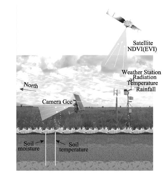
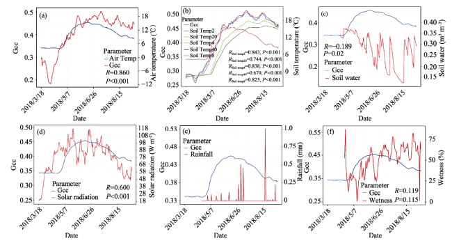
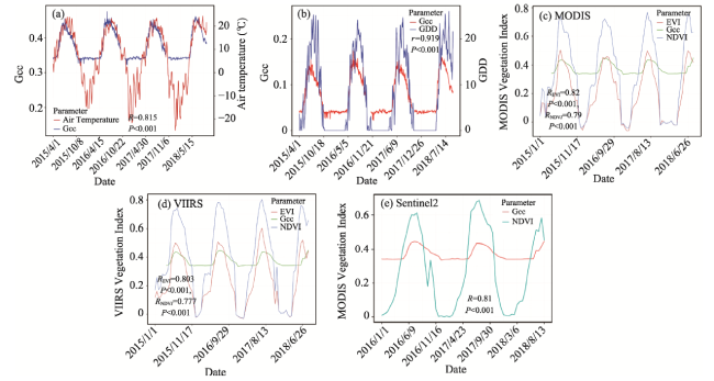
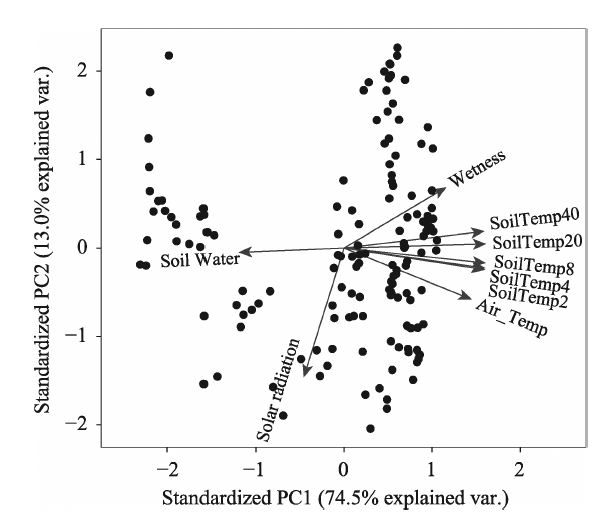
Near-surface remote sensing (e.g., digital cameras) has played an important role in capturing plant phenological metrics at either a focal or landscape scale. Exploring the relationship of the digital image-based greenness index (e.g., Gcc, green chromatic coordinate) with that derived from satellites is critical for land surface process research. Moreover, our understanding of how well Gcc time series associate with environmental variables at field stations in North American prairies remains limited. This paper investigated the response of grass Gcc to daily environmental factors in 2018, such as soil moisture (temperature), air temperature, and solar radiation. Thereafter, using a derivative-based phenology extraction method, we evaluated the correspondence between key phenological events (mainly including start, end and length of growing season, and date with maximum greenness value) derived from Gcc, MODIS and VIIRS NDVI (EVI) for the period 2015-2018. The results showed that daily Gcc was in good agreement with ground-level environmental variables. Additionally, multivariate regression analysis identified that the grass growth in the study area was mainly affected by soil temperature and solar radiation, but not by air temperature. High frequency Gcc time series can respond immediately to precipitation events. In the same year, the phenological metrics retrieved from digital cameras and multiple satellites are similar, with spring phenology having a larger relative difference. There are distinct divergences between changing rates in the greenup and senescence stages. Gcc also shows a close relationship with growing degree days (GDD) derived from air temperature. This study evaluated the performance of a digital camera for monitoring vegetation phenological metrics and related climatic factors. This research will enable multiscale modeling of plant phenology and grassland resource management of temperate prairie ecosystems.
ZHOU Yuke . Greenness Index from Phenocams Performs Well in Linking Climatic Factors and Monitoring Grass Phenology in a Temperate Prairie Ecosystem[J]. Journal of Resources and Ecology, 2019 , 10(5) : 481 -493 . DOI: 10.5814/j.issn.1674-764X.2019.05.003
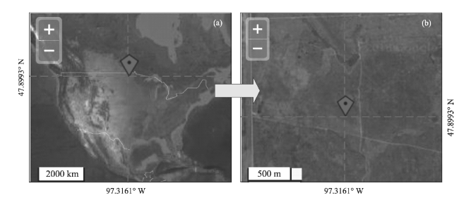
Fig. 2 Overview of the Oakville Prairie Biological Field Station (a) and its surrounding land cover (b) |
Table 1 Meta data for Oakville Prairie field station |
| Location | Elevation | Camera description | Camera orientation | Vegetation type | North America ecoregion | Dominant species |
|---|---|---|---|---|---|---|
| 47.8993°N, 97.3161°W | 268 m | StarDot NetCam SC | North | Grassland | No. 9 Temperate prairies | Andropogon gerardii, Distichlis spicata, Muhlenbergia richardsonis |
Table 2 Description of the datasets |
| Data name | Start date | End date | Frequency | Integrated frequency | Spatial scope |
|---|---|---|---|---|---|
| Gcc | 2015-4-1 | 2018-9-11 | 30 min | Daily | Landscape scale |
| Modis NDVI(EVI) | 2015-1-1 | 2018-9-11 | 16 day | Semimonthly | 2.5 km×2.5 km |
| VIIRS NDVI(EVI) | 2015-1-1 | ||||
| Air Temperature (Oakville) | 2018-3-18 | 2018-9-11 | 15 min | Daily | Point |
| Air Temperature (Grand Forks) | 2015-4-1 | 2018-9-11 | Daily | Daily | Point |
| Precipitation (Oakville) | 2018-3-18 | 2018-9-11 | 15 min | Daily | Point |
| Precipitation (Grand Forks) | 2015-4-1 | 2018-9-11 | Daily | Daily | Point |
| GDD (Grand Forks) | 2015-4-1 | 2018-9-11 | Daily | Daily | Point |
| Soil Water Content | 2018-3-18 | 2018-9-11 | 15 min | Daily | Point |
| Soil Temperature 2" | 2018-3-18 | 2018-9-11 | 15 min | Daily | Point |
| Soil Temperature 4" | 2018-3-18 | 2018-9-11 | 15 min | Daily | Point |
| Soil Temperature 8" | 2018-3-18 | 2018-9-11 | 15 min | Daily | Point |
| Soil Temperature 20" | 2018-3-18 | 2018-9-11 | 15 min | Daily | Point |
| Soil Temperature 40" | 2018-3-18 | 2018-9-11 | 15 min | Daily | Point |
Table 3 Statistical results of stepwise regression coefficients |
| Coefficients | Estimate | Std. error | t value | Pr (>|t|) |
|---|---|---|---|---|
| Intercept | 3.132e-01 | 7.881e-03 | 39.798 | < 2e-16 *** |
| Solar | 2.527e-04 | 5.277e-05 | 4.788 | 4.28e-06 *** |
| SoilTemp4 | -8.647e-03 | 3.546e-03 | -2.439 | 0.0160 * |
| SoilTemp8 | 8.264e-03 | 4.011e-03 | 2.061 | 0.0412 * |
| SoilTemp20 | 3.756e-02 | 2.804e-03 | 13.396 | < 2e-16 *** |
| SoilTemp40 | -3.677e-02 | 2.066e-03 | -17.801 | < 2e-16 *** |
| Soil Water | 6.107e-02 | 1.167e-02 | 5.232 | 6.10e-07 *** |
Note: Significance codes: *** means P<0.001, ** means P< 0.01 and * means P< 0.05 |
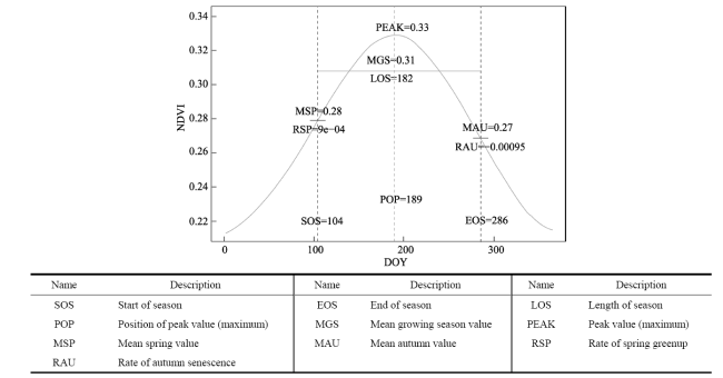
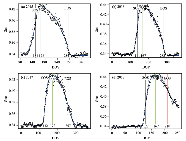
Table 4 Phenological metrics derived from daily Gcc. The unit of SOS, EOS, POP is day of year (DOY) |
| Year | SOS | EOS | LOS | POP | MGS | RSP | RAU | PEAK | MSP | MAU | |||
|---|---|---|---|---|---|---|---|---|---|---|---|---|---|
| 2015 | 151 | 284 | 133 | 172 | 0.402 | 0.003 | -0.0014 | 0.426 | 0.398 | 0.350 | |||
| 2016 | 141 | 283 | 142 | 167 | 0.412 | 0.0036 | -0.0017 | 0.438 | 0.3981 | 0.352 | |||
| 2017 | 132 | 257 | 125 | 172 | 0.411 | 0.0032 | -0.0013 | 0.427 | 0.376 | 0.374 | |||
| 2018 | 127 | 210 | 83 | 167 | 0.438 | 0.005 | -0.0013 | 0.451 | 0.386 | 0.420 | |||
| Mean | 137 | 258 | 120 | 169 | 0.416 | 0.0037 | -0.0014 | 0.4355 | 0.389 | 0.374 | |||
Table 5 Phenological metrics derived from various vegetation indices (with a temporal frequency of 16 days). The unit of SOS, EOS, POP is day of year (DOY), and the unit of LOS is Days. |
| Year | VI | SOS | EOS | LOS | POP | MGS | RSP | RAU | Peak | MSP | MAU |
|---|---|---|---|---|---|---|---|---|---|---|---|
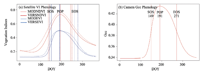
| 2015 | Gcc | 149 | 271 | 122 | 191 | 0.420 | 0.003 | -0.001 | 0.434 | 0.388 | 0.378 |
| MODNDVI | 143 | 243 | 100 | 194 | 0.661 | 0.007 | -0.004 | 0.732 | 0.499 | 0.584 | |
| MODEVI | 151 | 261 | 110 | 190 | 0.444 | 0.010 | -0.004 | 0.504 | 0.324 | 0.332 | |
| VIIRSNDVI | 137 | 250 | 113 | 194 | 0.690 | 0.006 | -0.004 | 0.761 | 0.541 | 0.599 | |
| VIIRSEVI | 142 | 278 | 136 | 192 | 0.445 | 0.009 | -0.005 | 0.495 | 0.323 | 0.317 | |
| Dev | 0.042 | 0.05 | 0.07 | 0.005 | 0.250 | 0.625 | 0.760 | 0.30 | 0.08 | 0.170 | |
| 2016 | Gcc | 152 | 340 | 188 | 200 | 0.406 | 0.003 | -0.001 | 0.447 | 0.393 | 0.348 |
| MODNDVI | 108 | 338 | 230 | 221 | 0.562 | 0.005 | -0.007 | 0.721 | 0.372 | 0.209 | |
| MODEVI | 133 | 312 | 179 | 221 | 0.382 | 0.003 | -0.004 | 0.462 | 0.274 | 0.22 | |
| VIIRSNDVI | 102 | 329 | 227 | 214 | 0.628 | 0.005 | -0.007 | 0.79 | 0.419 | 0.284 | |
| VIIRSEVI | 146 | 265 | 119 | 205 | 0.451 | 0.004 | -0.004 | 0.51 | 0.350 | 0.354 | |
| Dev | 0.25 | 0.09 | 0.005 | 0.07 | 0.20 | 0.29 | 0.82 | 0.28 | 0.11 | 0.30 | |
| 2017 | Gcc | 176 | 295 | 119 | 213 | 0.423 | 0.003 | -0.001 | 0.438 | 0.393 | 0.391 |
| MODNDVI | 128 | 296 | 168 | 214 | 0.620 | 0.005 | -0.007 | 0.745 | 0.444 | 0.368 | |
| MODEVI | 142 | 279 | 137 | 210 | 0.408 | 0.004 | -0.005 | 0.481 | 0.301 | 0.27 | |
| VIIRSNDVI | 120 | 278 | 158 | 199 | 0.670 | 0.006 | -0.005 | 0.777 | 0.456 | 0.525 | |
| VIIRSEVI | 145 | 256 | 111 | 200 | 0.516 | 0.006 | -0.005 | 0.591 | 0.379 | 0.405 | |
| Dev | 0.32 | 0.06 | 0.17 | 0.04 | 0.24 | 0.43 | 0.82 | 0.32 | 0.05 | 0.003 |
| [1] |
|
| [2] |
|
| [3] |
|
| [4] |
|
| [5] |
|
| [6] |
|
| [7] |
|
| [8] |
|
| [9] |
|
| [10] |
|
| [11] |
|
| [12] |
|
| [13] |
|
| [14] |
|
| [15] |
|
| [16] |
|
| [17] |
|
| [18] |
|
| [19] |
|
| [20] |
|
| [21] |
|
| [22] |
|
| [23] |
|
| [24] |
|
| [25] |
|
| [26] |
|
| [27] |
|
| [28] |
|
| [29] |
|
| [30] |
|
| [31] |
|
| [32] |
|
| [33] |
|
| [34] |
|
| [35] |
|
| [36] |
|
| [37] |
|
| [38] |
|
| [39] |
|
| [40] |
|
| [41] |
|
| [42] |
|
/
| 〈 |
|
〉 |