Resource Management

Sampling Size Requirements to Delineate Spatial Variability of Soil Properties for Site-Specific Nutrient Management in Rubber Tree Plantations

  • LIN Qinghuo , 1, 2 ,
  • LI Hong , 3, 4, * ,
  • LI Baoguo 2 ,
  • LUO Wei 1 ,
  • LIN Zhaomu 1 ,
  • CHA Zhengzao 1 ,
  • GUO Pengtao 1
Expand
  • 1. Rubber Research Institute, Chinese Academy of Tropical Agricultural Sciences, Haikou 571101, China
  • 2. Department of Soil and Water Sciences, China Agricultural University, Beijing 100193, China
  • 3. Haikou Cigar Research Institute, China Tobacco Corporation Hainan Provincial Bureau, Haikou 571100, China
  • 4. Environment and Plant Protection Institute, Chinese Academy of Tropical Agricultural Sciences, Haikou 571101, China
*Corresponding author: LI Hong, E-mail:

First author: LIN Qinghuo, E-mail:

Received date: 2018-11-07

  Accepted date: 2019-01-30

  Online published: 2019-07-30

Supported by

Foundation: National Key Research and Development Program of China (2018YFD0201100)

Foundation for China Agriculture Research System (CARS-34)

Fundamental Scientific Research Funds for Chinese Academy of Tropical Agricultural Sciences (1630022017007).

Copyright

All rights reserved

Abstract

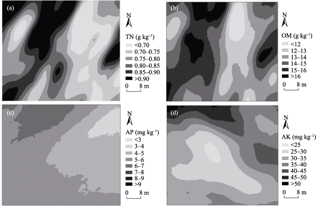
Site-specific nutrient management is an important strategy to promote sustainable production of rubber trees in order to obtain high yields of natural rubber. Making effective nutrient management decisions for rubber trees depend on knowing the spatial variations of soil fertility properties in advance. In this study the Kriging geostatistical method was used to examine the spatial variability of soil total nitrogen (TN), organic matter (OM), available phosphorus (AP) and available potassium (AK) in a typical hilly rubber tree plantation in Hainan, China. The spatial variability of the soils was small for the TN and OM and had medium variability for the AP and AK variables. Anisotropic semivariograms of all soil properties revealed that elevation and building contour ledge can profoundly affect the spatial variability of soil properties in the plantation, except for the AK variable. Soil samples had to be collected in alignment with the direction of elevation and perpendicular to the direction of building contour ledges, which was needed to obtain more reliable information within the study area in the rubber tree plantation. In formulating a sample scheme for AK, the distribution features of the soil’s parent material should be considered as the influence factor in the study field. The Kriging method used to guide the soil sampling for spatial variability dertermination of soil properties was about 2-5 times more efficient than the classic statistical method.

Cite this article

LIN Qinghuo , LI Hong , LI Baoguo , LUO Wei , LIN Zhaomu , CHA Zhengzao , GUO Pengtao . Sampling Size Requirements to Delineate Spatial Variability of Soil Properties for Site-Specific Nutrient Management in Rubber Tree Plantations[J]. Journal of Resources and Ecology, 2019 , 10(4) : 441 -450 . DOI: 10.5814/j.issn.1674-764X.2019.04.011

1 Introduction

Rubber tree (Hevea brasiliensis (Wild.) Muell.-Arg.), a member of the family Euphorbiaceae, originated in the Amazon basin, is the main source of natural latex. The increased demands for natural rubber worldwide require increasing production of rubber latex. However, the available areas under rubber tree cultivation for latex production were only about 10.3 million ha in 2009 in all tropical zones globally (Lacote et al., 2010). The world rubber production was estimated to be about 11.6 million tons in 2012, of which the production in Asia and Africa accounted for about 93% and the rest of the world represented only about 7% of total production (Irsg, 2013). Natural rubber has been a key product for many tropical countries in southeastern Asia, South America and Africa (Michels et al., 2012). In 2013, rubber plantations covered approximately 1.07 × 10⁴ ha in China and approximately half of the total plantation areas were located in Hainan island in southern China. Plantations of rubber trees form the largest type of artificial ecosystem on Hainan island (Lin et al., 2013).
Rubber trees are perennial plants and their latex is extracted using a multi-annual tapping system that allows trees to be productive for 15-30 years or longer (Michels et al., 2012). However, nutritional level degradation in intensive rubber plantations is a problem due to the long-term extraction of latex that exports many nutritional elements from the soil (Zhang et al., 2007). Thus, to maintain the sustainable growth of rubber trees and the high yields of natural rubber, it is necessary to apply chemical fertilizers based on site- specific nutrient management decisions during rubber production.
Site-specific nutrient management requires reliable information about the spatial variability of soil properties in order to make effective management decisions (Kerry and Oliver, 2003). Accurate mapping of soil properties is a critical constituent of successful site-specific agriculture, and is often obtained by the use of sample locations within the production areas (Li et al., 2014; Lin et al., 2013). The quality of mapping and the spatial distribution of soil properties depend on the accuracy of the interpolated values, which, in turn, depends on the initial sampling scheme (Shi et al., 2000). Recurring questions confronting any research effort concern dilemmas about how many soil samples should be taken and where in the study area they should be taken from (Di et al., 1989). These questions exist not only in studies of site-specific nutrient management for rubber trees, but also in other soil and ecological studies (Dale et al., 1991; Vasu et al., 2017).
Effective sampling strategies should identify both the sampling sizes and spatial distributions of sampling locations in order to be cost-effective in terms of time and labor (De Caires et al., 2014; Gao and Shao, 2012). The variability of soil properties within study units has often been described using classic statistical methods (Adachi et al., 2005; Garten et al., 2007; Metcalfe et al., 2008). Classical statistics assume that variations of soil properties within sampling units are randomly or spatially uncorrelated and that the mean value of samples is the best estimator of soil properties at any location within the sampling units (Cochran, 1977). However, many studies have shown that soil properties often tend to be spatially correlated within study areas (Di et al., 1989; Goovaerts, 1997; Oliver and Webster, 2014; Webster and Oliver, 2001). Geostatistics provides a tool for improving sampling design by utilizing the spatial dependence of soil properties within sampling units (Di et al., 1989; Matheron, 1965). Some have suggested that actual efficiency achieved may be three to nine times greater than the values estimated by classic statistical methods (Mcbratney and Webster, 1983).
Rubber plantations are usually located in hilly areas and the management practices used for rubber trees have changed little over time in Hainan (Dong et al., 2012; Lin et al., 2013). Under these circumstances, how many soil sample sites and where these sites are located in the rubber plantations must be determined to make effective site- specific nutrient management decisions. These decisions are important and must be made efficiently because rubber tree plantations are long-term production systems that are time intensive and have high labor costs (Lin et al., 2016). To address these issues, this study used dense sampling to explore and analyze the spatial structure of soil chemical properties at a typical rubber tree plantation. The objectives of this study were to: 1) evaluate the spatial variability of selected chemical properties of soil in a rubber plantation; 2) compare the sampling sizes needed to estimate the means of the selected soil properties within specified intervals using the classic statistical method and the geostatistics method; and 3) use different sampling strategies to determine the optimal sampling patterns for delineating the spatial variability of soil properties for site-specific nutrient management of rubber trees.

2 Materials and methods

2.1 Site description

The study was conducted at a typical rubber tree plantation in Yangjiang State Farm located in Qiongzhong, Hainan island, China. The climate in the region is classified as a tropical monsoon: the mean annual precipitation is 2000 mm with about 90% of the annual rainfall occurring from intense rainstorms in the period from May to October; the mean annual potential evapotranspiration is 1780 mm; and the annual mean temperature is 23.5°C. The soil, developed mainly from granites, is classified as a Udic Ferralosol according to the World Reference Base for Soil Resources (FAO, 1998).
The area selected for this study was a zone of 4200 m2, approximately 70 m west to east and 60 m north to south in extent. The elevation of the rubber tree (Hevea brasiliensis (Wild.) Muell.-Arg.) plantation is 250 m in the east and 245 m in the west, with an average slope of 8°. The rubber trees are clones of PR107 planted in 1993, with a height of about 10 m. There was a total of 231 rubber trees within the experimental plot and the center point of the geo-coordinates was 19°18′47.8″N and 109°45′52.0″E. The tree spacing was 7 m between rows, which ran from west to east, and 3 m along the rows. Contour ledges were located in a north to south direction in each row to prevent soil erosion from rainfall. The study area was mainly covered by a tropical kudzu (Pueraria phaseoloides Benth var. javanica Baker) and calopo (Calopogonium mucunoides Desv).
Conventional fertilization caves used for the application of fertilizer were located between two rows with a vertical distance of 1.5 m from the rhizome neck (the stump place of rubber trees). Subsoils dug from the fertilization caves were used to preserve the outer edge of the contour ledge (a contour barrier built with subsoil to prevent soil erosion). The shrub and ruderal zones were in the middle of the same row, where there was the free land of approximately 3 m in width between the adjacent rubber-planting strips with vegetation growth for controlling nature. The existing fertilization model used an annual amount of 2.0 kg mixed chemical fertilizers for each tree in the area; the fertilizer compound was composed of 0.7 kg urea (CO(NH2)2), 1.0 kg monocalcium phosphate (Ca(H2PO4)2) and 0.3 kg potassium chlorine (KCl). Three applications were scheduled, in the middle of March, June and September each year. Half of the total fertilizers were applied in March and the rest was split equally between the later two applications (Lin et al., 2013).

2.2 Soil sampling and analyses

A total of 100 sampling sites were located in equivalent rectangular grids (Fig. 1). The dimension of each rectangular grid for sampling was 6 m × 7 m. A regular grid sampling strategy had been proven to be more effective in predicting spatial heterogeneity than randomized sampling (Hirzel and Guisan, 2002). On August 28th, 2011, five subsamples of the topsoil (0-20 cm) in the shrub and ruderal zones with opposite angles within a 1 m radius were collected from each rectangular sampling site using an auger 8 cm in diameter. Subsamples were mixed thoroughly to obtain approximately 1 kg of composite samples. Root tissue, grass and leaves in the soil samples were discarded. The soil samples were air-dried, ground and then passed through a 2 mm sieve.
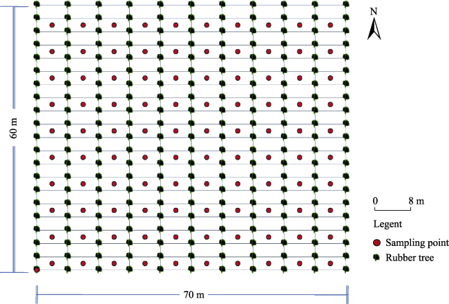
Fig. 1 Sampling sites (100 sites) in the rubber tree plantation (4200 m2)
Note: The dimension of each rectangle grid for sampling was 6 m × 7 m.
The chemical properties of the soil were analyzed using the standard test methods (Bao, 2000). Organic matter (OM) in the soil was determined using the potassium dichromate-wet combustion procedure. Total nitrogen (TN) was determined using the Kjeldahl distillation method. Available phosphorus (AP) was extracted using a NH4F-HCl solution. Available potassium (AK) was extracted using 1.0 mol/L CH3COONH4 and then measured with an atomic absorption spectrometer.

2.3 Design of different sampling combinations

Four sampling combinations were used to compare the accuracy of different sampling strategies. Two sampling combinations were sampled at 50 sites on rectangular grids of 6 m × 14 m and 12 m × 7 m, respectively. The other two sampling combinations, with grids of 6 m × 21 m and 18 m × 7 m, were used at 40 sites (Fig. 2).
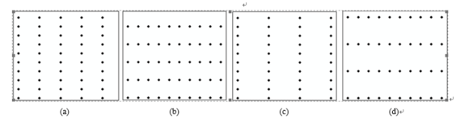
Fig. 2 Sampling points of different sampling strategies
Note: (a) sampling spacing 6 m × 14 m, 50 sampling numbers; (b) sampling spacing 12 m ×7 m, 50 sampling numbers; (c) sampling spacing 6 m × 21 m, 40 sampling numbers; (d) sampling spacing 18 m × 7 m, 40 sampling numbers.

2.4 Statistical method

2.4.1 Sample size estimate by classic statistical method
In classic statistics, the number of samples needed for estimating the mean value of a soil property can be determined from the following formula (Cochran, 1977):
$n=\frac{{{t}^{2}}{{_{(n-1,1-}}_{\alpha /2)}}{{s}^{2}}}{{{(x-\mu )}^{2}}}$ (1)
Where ${{t}_{(n-1,1-\alpha /2)}}$ is the t-test at the chosen level of confidence α, s2 is the variance, and (xu) is the acceptable error in the sample mean u. If n is larger than 10% of the population size (N), then fewer observations, i.e. ${n}'=n/$ $(1+n/N),$are sufficient to achieve the same confidence level and accuracy (Sachs, 1982).
2.4.2 Estimation of the sampling size by geostatistical method
In the geostatistics method, the semivariogram illustrates the relationship between the semivariance of samples and the
distance or the lag separating them. The semivariance $\gamma (h)$ is defined as (Matheron, 1965):
$\gamma (h)=\frac{1}{2N(h)}\sum\limits_{i=1}^{N(h)}{[Z ({{x}_{i}}+h)}-Z ({{x}_{i}}){{]}^{2}}$ (2)
Where h is the lag distance separating pairs of points, $Z({{x}_{i}})$ is the value of the regionalized variable of interest at location xi, and $Z({{x}_{i}}+h)$. is the value at the location ${{x}_{i}}+h$, and$N(h)$is the number of pairs separated by the lag distance h.
The semivariogram for all soil properties was produced by plotting all the semivariances versus their lag distances. Different theoretical semivariogram models were used to fit the calculated values, and the model with the best fitting value was generated. Cross-validation method was used to validate the parameters of the model based on three statistical measurements: the mean prediction error (ME), root- mean-square error (RMSE), and the root-mean-square standardized prediction error (RMSSE) (Goovaerts, 1997). If the ME is closest to 0, the RMSE is the smallest value and the RMSSE is closest to 1, the experimental semivariogram models have good predictive capability and should be selected (Piccini et al., 2014). The most popular function is the spherical-plus-nugget model and the expression in equation is:\[\gamma (h)=\left\{ \begin{array}{*{35}{l}}0 \\{{C}_{0}}+{{C}_{1}}\left[ 1.5h/A-0.5{{(h/A)}^{3}} \right] \\{{C}_{0}}+{{C}_{1}} \\\end{array} \right.\] $\begin{array}{*{35}{l}}h=0 \\0<h<A \\h\ge A \\\end{array}$ (3)
Where ${{C}_{0}}$ is nugget variance, and represents the uncorrelated variation at the scale of sampling, arising from the random components like measurement error and micro-scale processes; ${{C}_{1}}$ is the spatially correlated variance, representing continuity, arising from the spatial autocorrelation; ${{C}_{0}}+{{C}_{1}}$ estimates the variance of the random process and is known as the “sill” equivalent to the population variance; $A$ is the limit of the spatial correlation distance (or range).
The maximum lag distance is independent of the direction; it is isotropic. If the spatial correlation varies with the direction and distance, it is anisotropic. In many instances, variation is anisotropic. If it is disregarded, the result may give misleading views of the true situation (Oliver and Webster, 2014). When the anisotropy is geometric (the same sill is present in all directions but the range is changed with different directions), a simple linear transformation of the spatial coordinates will make the variation isotropic. The equation for the transformation is as follows:
$A=\sqrt{A_{1}^{2}\times \left[ \text{co}{{\text{s}}^{2}}\left( \theta -\varphi \right) \right]+A_{2}^{2}\times \left[ \text{si}{{\text{n}}^{2}}\left( \theta -\varphi \right) \right]}$ (4)
Where A1 is the range parameter for the major axis$(\varphi )$, and A2 is the range parameter for the minor axis$(\varphi +90)$, $\varphi $ is the angle of maximum variation, and $\theta $ is the direction of the lag. The anisotropy ratio ($\kappa $) is the ratio of the major to the minor axis, and it indicates that the degree of variation at a lag distance of $h$ in the major axis is the same as that of a lag distance of $\kappa h$ in the minor axis direction. The anisotropy ratio is determined as:
$\kappa ={{A}_{1}}/{{A}_{2}}$ (5)
When the experimental semivariogram increases without bounds ever more steeply as the lag distance increases, the trend (a gradual variation in space) should be taken into account (Oliver and Webster, 2014). In this case, the trend was ignored, based on the feature shown in Fig.3. The semivariogram model is used in the subsequent phase, geostatistical interpolation or kriging. Kriging calculates linear unbiased estimates at non-sampled points as a weighted average of the neighboring sampled points. The interpolated value,${{Z}^{*}}({{x}_{0}})$, of the property at location ${{x}_{0}}$ is calculated as follows:
${{Z }^{*}}({{x}_{0}})=\sum\limits_{i=1}^{n}{{{\lambda }_{i}}\times }Z ({{x}_{i}})$ (6)
Where $Z({{x}_{i}})$ is the value of Z at the sampling point, and ${{\lambda }_{i}}$ are the weights assigned to each $Z({{x}_{i}})$. The weights are constrained to sum to 1, thereby assuring an unbiased estimate.
The estimation variance, ${{\sigma }^{2}}(B)$, often called the kriging variance, can itself be estimated by the following expression (Mcbratney et al., 1981):
$\sigma _{{}}^{2}(B)=\sum\limits_{i=1}^{n}{{{\lambda }_{i}}}\bar{\gamma }({{x}_{i}},B)+\psi (B)-\bar{\gamma }(B,B)$ (7)
Where $\bar{\gamma }({{x}_{i}},B)$ is the average semivariance between observation points ${{x}_{i}}$ in the neighborhood and all the points within the block $B$, $\bar{\gamma }(B,B)$ are the average semivariance between all points with the block (i.e., the within-block variance), and $\psi (B)$ is the Lagrange parameter associated with the minimization process.
2.4.3 Comparison of different sampling combinations
Four new sample combinations were obtained after rows or columns of sampling points were removed alternatively (Fig. 2). Soil properties of the four new sampling combinations were subjected to ordinary kriging interpolation. The mean values predicted at each sampling point in each of the new four sampling combinations were then compared with those observed values for the original sample combinations (Fig. 1).
Various validation indices can be used as a measure for prediction quality, of which the most common is the RMSE (Bishop and Mcbratney, 2001), which is calculated by using equationas follows:
$RMSE=\sqrt{\frac{1}{n}\sum\limits_{i=1}^{n}{{{\left[ Z ({{x}_{i}})-{{Z }^{*}}({{x}_{i}}) \right]}^{2}}}}$ (8)
Where $Z({{x}_{i}})$= the predicted value, ${{Z}^{*}}({{x}_{i}})$= the actual observed value.
A further measure of a goodness-of-prediction ($G$) was used to investigate the accuracy of each combination (Gao and Shao, 2012; Gotway et al., 1996). Values for $G$ were computed using the equation (9):
$G=\left\{ 1-\left[ {\sum\limits_{i=1}^{n}{{{\left( Z ({{x}_{i}})-{{Z }^{*}}({{x}_{i}}) \right)}^{2}}}}/{\sum\limits_{i=1}^{n}{{{\left( Z ({{x}_{i}})-\bar{Z }({{x}_{i}}) \right)}^{2}}}}\; \right] \right\}\times 100$ (9)
Where $Z({{x}_{i}})$ is the predicted value at point $i$, ${{Z}^{*}}({{x}_{i}})$ is the observed value at point $i$, and $\bar{Z}({{x}_{i}})$ is the sample arithmetic mean. A $G$ value of 100 indicates perfect prediction corresponding to a $RMSE$ = 0, while the negative values indicate that using the arithmetic sample mean is more reliable than the tested predictor is.

2.5 Data statistics and mapping

The normal distributions of all the samples were tested using the one-sample Kolmogorov-Simirnov test (K-S) (P < 0.05). The descriptive statistics (determination of means, standard deviations, coefficient of variation, and kurtosis, etc.) of all soil datasets were obtained using the Statistical Program for Social Sciences (SPSS) 13.0. Geostatistical analysis consisting of variogram calculation, cross-validation, kriging and mapping were performed using the geostatistical analyst extension of ArcGIS 9.3 (ESRI, USA).

3 Results and discussion

3.1 Exploratory data analysis

The geometric means of TN, OM and AK concentrations in the soil were 0.79 g kg-1, 14.29 g kg-1 and 34.68 mg kg-1, respectively (Table 1). These were slightly lower than the critical values required for maintaining median latex yield production (Table 2). The soil AP concentration was relatively higher than the critical value of 5 mg kg-1 needed for the median yield growth. Soil spatial variability was small for TN and OM with CV values of 14.64% and 13.95%, based on the variability assessment by Da Silva et al. (2009). The available soil chemical properties exhibited a medium variability (CVs ranged from 28.68% for AP to 30.77% for AK), with approximately a threefold variation range between maximum and minimum concentrations. The skewness, kurtosis and Kolmogorov-Smirnov (K-S) tests showed that all the soil properties belonged to the normal distributions (Pk-s > 0.05) (Table 1).
Table 1 Statistical parameters for selected chemical properties of soil in a rubber plantation (100 samples in total)
Soil properties Mean Range SD CV(%) Skew Kurt PK-S*
TN(g kg-1) 0.79 0.48-1.13 0.12 14.64 0.35 0.58 0.43
OM(g kg-1) 14.29 8.44-19.64 1.99 13.95 0.20 0.93 0.67
AP(mg kg-1) 5.20 2.52-9.46 1.49 28.68 0.58 -0.08 0.54
AK(mg kg-1) 34.68 20.01-62.39 10.67 30.77 0.93 0.17 0.10
Table 2 Classes of soil properties in a rubber plantation on Hainan Island (Lu, 1983)
Class TN(g kg-1) OM(g kg-1) AP(mg kg-1) AK(mg kg-1)
Abundant* >1.4 >25 >8 >60
Normal 0.8-1.4 20-25 5-8 40-60
Lack <0.8 <20 <5 <40

Note: * Abundant indicates high yield latex will be attained, with no additional application of fertilizers; Normal indicates median yield late will be attained, with a small amount of fertilizers needed; Lack indicates low yield latex will be attained, with the application of fertilizers having significant effects.

3.2 The spatial structural analysis of soil chemical properties

The best-fit variogram model was spherical to show theNote: TN, total nitrogen; OM, organic matter; AP, available phosphorous; AK, available potassium; Min, minimum value; Max, maximum value; SD, standard deviation, CV, coefficient of variation; Skew, skewness of raw data; Kurt, kurtosis of raw data. * means the normal distribution probability of Kolmogorov-Smironov (K-S) test, Pk-s > 0.05 indicates that the variable is normally distributed.spatial variability of all soil chemical properties (Table 3). The ME and RMSSE values approached 0 and 1, respectively, reflecting the high prediction capability of semivariogram models for all soil properties (Hu et al., 2014). The resulting semivariograms showed that the spatial variation of all variables for the studied field were anisotropic (Fig. 3), and it was indicated that the semivariogram could depend on both the distance and the direction of soil samplings.
Table 3 Semivariogram model of soil properties and their parameter in a rubber plantation
Variable Best model A1 (m) A2 (m) κ φ (°) C0 C1 C0/(C0+C1) Cross-validation indices
ME RMSE RMSSE
TN Spherical 52.93 16.93 3.13 20.5 4.18E-03 0.010 0.29 2.84E-03 0.087 0.975
OM Spherical 46.19 16.57 2.79 8.8 1.579 2.694 0.37 2.41E-02 1.737 1.06
AP Spherical 62.23 36.10 1.72 44.6 1.655 0.730 0.69 8.20E-04 1.439 1.028
AK Spherical 52.86 23.98 2.20 286.2 72.663 47.192 0.61 -3.47E-02 9.528 0.985

Note: A1, the range parameter for the major axis of soil properties; A2, the range parameter for the minor axis of soil properties; κ, the anisotropic ratio, A1/A2; φ, azimuth angle of the major axis, measured in degrees clockwise from the positive north direction; ME, mean error, should be near zero for a good prediction; RMSE, root-mean-square error, should be small for a good prediction; RMSSE, root-mean-square standardized error, should be close to 1 for a good prediction.

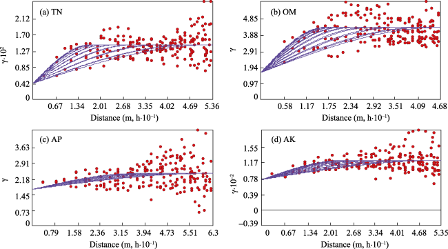
Fig. 3 Anisotropic semivariogram models for the selected soil properties in a rubber plantation. Chemical properties of soil included total nitrogen (TN); organic matter (OM); available phosphorous (AP); and available potassium (AK).
The range values show that the variables were spatially continuous for a certain distance and then became constant. Variations of range values in different directions reflected the variations of this extent in different directions. The spatial correlation ranges of TN, OM, AP and AK in the minor axis were 16.93, 16.57, 36.10 and 23.98 m, respectively, while the corresponding values in the major axis were 52.93, 46.19, 62.23 and 52.86 m, respectively (Table 3). The azimuth angle of the major axis for TN, OM and AP concentrations deviated from the east-west (E-W) direction, which indicated higher ranges in the north-south (N-S) direction, and lower ranges in the E-W direction (Table 3). The anisotropy ratios for TN, OM, AP and AK variables were 3.13, 2.79, 1.72 and 2.20, respectively. It was suggested that the direction of soil sampling could affect the spatial structure analysis for the chemical properties being determined.
The nugget to sill ratio, as shown in Table 3, is commonly selected to express the short-distance autocorrelation of regionalized variables. A low value of nugget to sill ratio indicates a high spatial autocorrelation or a spatial continuity over short distances (Oliver and Webster, 2014). In this study, the nugget to sill ratios for TN, OM, AP and AK were 0.29, 0.37, 0.69 and 0.61, respectively. All the values of the nugget to sill ration were between 0.25 and 0.75, therefore all the variables have a medium spatial correlation (Cambardella et al., 1994). The nugget to sill ratios for TN and OM were smaller than 50%, indicating that the spatial heterogeneity is mainly due to systematic variability. For both AP and AK, the nugget to sill ratios was more than50%, showing that they have weak spatial correlations.

3.3 The spatial distribution features of soil chemical properties

The TN, OM and AP variables showed a similar distributional trend (Fig. 4), generated by using the ordinary kriging method based on the fitted semivariogram modes. The distribution trends were with lower concentrations in the eastern regions but higher contents in the western regions where the elevation was relatively low. These trends were in accordance with the basic fact that more fine soil particles are packed in low elevation areas. However, the TN, OM and AP concentrations were relatively homogeneous in the N-S direction, which might be due to the building of the contour ledge.
Fig. 4 Anisotropic semivariogram models for the selected soil properties in a rubber plantation. Soil chemical properties included total nitrogen (TN); organic matter (OM); available phosphorous (AP); and available potassium (AK).
The AK concentrations were lower in the middle area, which might be due to the parent materials in the rubber tree plantation. The minerals quartz and K-feldspar that dominate ordinary granites are generally rich in potassium (K) and sodium (Na) (Wang et al., 2013). Therefore, the granites in the middle plantation areas should affect the spatial distribution of the AK variable. Also, all the variables showed the most continuous distribution along their corresponding azimuth angles of the major axis (Fig. 4). These were measured in degrees clockwise from the positive north direction.

3.4 Sampling size estimated by classic and geostatistic methods

The standard error for each soil property derived from kriging and the classic statistical approach was plotted against the number of observations (Fig. 5). The kriging standard error is considerably lower than that estimated by the classic method for the same number of observations. Kriging therefore requires fewer observations than those that are needed for the classic statistical method to achieve the same level of precision (Table 4). The use of kriging results in sample efficiency two to five fold greater than that of the classic statistical method in this study. These results are similar to those obtained by Mcbratney and Webster (1983), who claimed the use of kriging resulted in a three to nine fold gain in efficiency. These results demonstrate the fact that kriging takes into account the spatial dependence between observations in the study area, whereas the classic statistical theory does not take the spatial correlation and relative positions of sampling locations into account (Di et al., 1989).
Table 4 Estimated sample sizes (numbers) to obtain mean values within ±5% and ±10% of classic and Kriging methods
Variable ±5%* ±10%
SD Classic Kriging SD Classic Kriging
TN 0.04 27 9 0.08 10 2
OM 0.72 25 9 1.44 10 2
AP 0.26 57 29 0.52 26 8
AK 1.73 60 32 3.47 29 9

Note: * Within the certain error of the true population means.

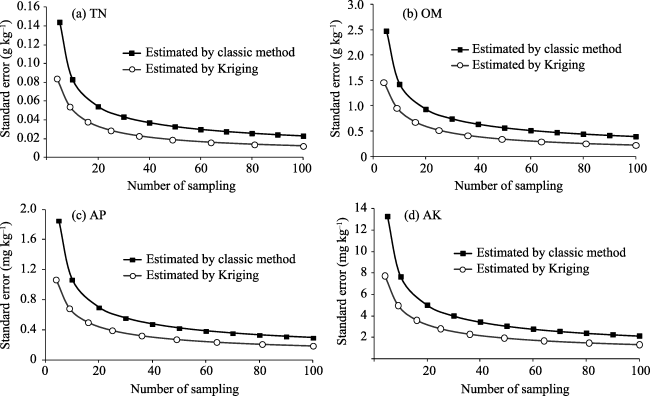
Fig. 5 Kriging and classic statistical standard errors in relation to sample sizes for estimating chemical properties of soil at a rubber plantation. Soil chemical properties included: (a) TN, total nitrogen; (b) OM, organic matter; (c) AP, available phosphorous; (d) AK, available potassium.

3.5 Comparisons of the prediction quality obtained by different sampling combinations

The influences of sample number and sampling patterns on kriging interpolation, assessed using four different subsets of data from the original soil property datasets, were different (Fig. 2). The RMSE and $G$tests showed how sample combinations had interpolated mean values closer to those (mean interpolated values) for the original datasets (Table 5). The $G$values of all sampling combinations were positive and the RMSE approached zero, indicating that the maps obtained from the interpolated data are more accurate than a field management average (Kravchenko, 2003).
Table 5 Test results of soil properties for various sampling strategies
Samplestrategy * Sample
number
TN OM AP AK
RMSE G RMSE G RMSE G RMSE G
A 50 0.07 61.09 1.27 58.78 1.08 46.71 6.75 59.58
B 50 0.07 64.61 1.19 63.98 1.03 52.30 7.57 49.19
C 40 0.08 47.51 1.47 44.80 1.18 36.47 7.98 43.57
D 40 0.08 48.37 1.44 47.09 1.21 33.58 9.30 23.27

* A: sampling spacing of 6 m × 14 m, sampling number of 50;
B: sampling spacing of 12 m × 7 m, sampling number of 50;
C: sampling spacing of 6 m × 21 m, sampling number of 40;
D: sampling spacing of 18 m × 7 m, sampling number of 40.
RMSE, root mean square error, the smallest is the best prediction; G, goodness for prediction, G values of 100 represent a prefect prediction.

As the sample size increased, the interpolation accuracy improved (Marques Jr et al., 2014). Therefore the sample size of 50 (Fig. 2a and Fig. 2b) was more accurate than that with the sample size of 40 (Fig. 2c and Fig. 2d) based on the values of both G and the RMSE (Table 5). However, it is not only sample size that needs to be considered. Sample combinations or arrangements should also be considered when devising sampling schemes for mapping the distribution of soil properties. For example, although the sample number for the combinations shown in Fig. 2a and Fig. 2b were identical, the arrangement of sampling combinations in Fig. 2b gave a more accurate prediction than the combinations in Fig. 2a for the TN, OM and AP variables. This was probably due to the sampling arrangement of the data combinations (Fig. 2b), in which more soil samples were collected in the E-W direction where the spatial variability of TN, OM and AP were larger than in other directions. Similar results were found for the data combinations (Fig. 2c, Fig. 2d and Fig. 3).

4 Conclusions

Sampling locations for determining spatial variability of soil properties were significantly affected by site elevation. The Kriging method used to guide the soil sampling for spatial variability determination of soil properties was about 2-5 times more efficient than the classic statistical method. Nutrient management required the careful selection of farming operation type. More soil samples should be collected in alignment with the direction of elevation and perpendicular to the direction of building contour ledges to obtain reliable management information for use in rubber tree plantations. Because the parent materials of the soils in the study area were granites, no significant correlation between AK and elevation or between AK and contour ledge was observed. Under this circumstance, the distribution features of the parent materials of the soils should be considered for the AK sample scheme. To achieve the desired precision, we can quantify the number of samples needed from graphs of standard error against sample size.
[1]
Adachi M, Bekku Y S, Konuma A, et al.2005. Required sample size for estimating soil respiration rates in large areas of two tropical forests and of two types of plantation in Malaysia.Forest Ecology and Management, 210(1-3): 455-459.

[2]
Bao S D.2000. Soil Agricultural Chemistry Analysis. Beijing: Agriculture Press. (in Chinese).

[3]
Bishop T F A, Mcbratney A B.2001. A comparison of prediction methods for the creation of field-extent soil property maps.Geoderma, 103(1): 149-160.

[4]
Cambardella C A, Moorman T B, Parkin T B,et al.1994. Field-Scale Variability of Soil Properties in Central Iowa Soils.Soil Science Society of America Journal, 58(5): 1501-1511.

[5]
Cochran W G.1977. Sampling Techniques, 3rd Edition. New York: John Wiley and Sons.

[6]
Da Silva B M C G, Ambrosano G M B, Flrio F M, et al.2009. Assessment of variability in experiments in the operative dentistry area applied to shear bond strength tests.Revista de Odontologia da UNESP, 38(2): 117-121.

[7]
Dale V H, Franklin R L A, Post W M,et al.1991. Sampling ecological information: Choice of sample size.Ecological Modelling, 57(1-2): 1-10.

[8]
De Caires S A, Wuddivira M N, Bekele I.2014. Spatial analysis for management zone delineation in a humid tropic cocoa plantation.Precision Agriculture,16(2): 129-147.

[9]
Di H J, Trangmar B, Kemp R.1989. Use of geostatistics in designing sampling strategies for soil survey.Soil Science Society of America Journal, 53(4): 1163-1167.

[10]
Dong J, Xiao X, Sheldon S, et al.2012. Mapping tropical forests and rubber plantations in complex landscapes by integrating PALSAR and MODIS imagery.ISPRS Journal of Photogrammetry and Remote Sensing, 74: 20-33.

[11]
FAO.1998. World reference base for soil resources. World Soil Resources Report No. 84, FAO, Rome.

[12]
Gao L, Shao M.2012. The interpolation accuracy for seven soil properties at various sampling scales on the Loess Plateau, China.Journal of Soils and Sediments, 12(2): 128-142.

[13]
Garten J C T, Kang S, Brice D J, et al.2007. Variability in soil properties at different spatial scales (1 m-1 km) in a deciduous forest ecosystem.Soil Biology and Biochemistry, 39(10): 2621-2627.

[14]
Goovaerts P.1997. Geostatistics for Natural Resources Evaluation. Oxford University Press, USA.

[15]
Gotway C A, Ferguson R B, Hergert G W, et al.1996. Comparison of kriging and inverse-distance methods for mapping soil parameters.Soil Science Society of America Journal, 60(4): 1237-1247.

[16]
Hirzel A, Guisan A.2002. Which is the optimal sampling strategy for habitat suitability modelling.Ecological Modelling, 157(2-3): 331-341.

[17]
Hu K, Wang S, Li H, et al.2014. Spatial scaling effects on variability of soil organic matter and total nitrogen in suburban Beijing. Geoderma, 226-227: 54-63.

[18]
Irsg.2013. Rubber Statistical Bulletin. International rubber study group,Singapore, 55.

[19]
Kerry R, Oliver M.2003. Variograms of Ancillary Data to Aid Sampling for Soil Surveys.Precision Agriculture, 4(3): 261-278.

[20]
Kravchenko A N.2003. Influence of Spatial Structure on Accuracy of Interpolation Methods.Soil Science Society of America Journal, 67(5): 1564-1571.

[21]
Lacote R, Gabla O, Obouayeba S,et al.2010. Long-term effect of ethylene stimulation on the yield of rubber trees is linked to latex cell biochemistry.Field Crops Research, 115(1): 94-98.

[22]
Li H, Bielder C, Payne W A, et al.2014. Spatial characterization of scaled hydraulic conductivity functions in the internal drainage process leading to tropical semiarid soil management.Journal of Arid Environments, 105: 64-74.

[23]
Lin Q H, Li H, Li B G, et al.2016. Assessment of spatial uncertainty for delineating optimal soil sampling sites in rubber tree management using sequential indicator simulation.Industrial Crops and Products, 91: 231-237.

[24]
Lin Q, Li H, Luo W, et al.2013. Optimal soil-sampling design for rubber tree management based on fuzzy clustering.Forest Ecology and Management, 308: 214-222.

[25]
Marques J J, Siqueira D S, Camargo L A,et al.2014. Magnetic susceptibility and diffuse reflectance spectroscopy to characterize the spatial variability of soil properties in a Brazilian Haplustalf. Geoderma, 219-220: 63-71.

[26]
Matheron G.1965. Les Variables Régionalisées et leur Estimation . Pairs:Masson.

[27]
Mcbratney A B, Webster R.1983. How many observations are needed for regional estimation of soil properties?Soil Science, 135(3): 177-183.

[28]
Mcbratney A B, Webster R, Burgess T M.1981. The design of optimal sampling schemes for local estimation and mapping of of regionalized variables—I: Theory and method.Computers & Geosciences, 7(4): 331-334.

[29]
Metcalfe D, Meir P, C Aragão L E O#magtechI#,et al.2008. Sample sizes for estimating key ecosystem characteristics in a tropical terra firme rainforest.Forest Ecology and Management, 255(3-4): 558-566.

[30]
Michels T, Eschbach J M, Lacote R,et al.2012. Tapping panel diagnosis, an innovative on-farm decision support system for rubber tree tapping.Agronomy for Sustainable Development, 32(3): 791-801.

[31]
Oliver M A, Webster R.2014. A tutorial guide to geostatistics: Computing and modelling variograms and kriging.Catena, 113: 56-69.

[32]
Piccini C, Marchetti A, Francaviglia R.2014. Estimation of soil organic matter by geostatistical methods: Use of auxiliary information in agricultural and environmental assessment.Ecological Indicators, 36: 301-314.

[33]
Sachs L.1982. Appalied Statistics. New York:Springer-Verlag, 706.

[34]
Shi Z, Wang K, Bailey J S, et al.2000. Sampling strategies for mapping soil phosphorus and soil potassium distributions in cool temperate grassland.Precision Agriculture, 2(4): 347-357.

[35]
Vasu D, Singh S K, Sahu N,et al.2017. Assessment of spatial variability of soil properties using geospatial techniques for farm level nutrient management.Soil and Tillage Research, 169: 25-34.

[36]
Wang R C, Xie L, Chen J, et al.2013. Tin-carrier minerals in metaluminous granites of the western Nanling Range (southern China): Constraints on processes of tin mineralization in oxidized granites.Journal of Asian Earth Sciences, 74: 361-372.

[37]
Webster R, Oliver M A.2001. Geostatistics for Environmental Scientists, 2nd ed. New York: John Wiley and Sons.

[38]
Zhang H, Zhang G L, Zhao Y G, et al.2007. Chemical degradation of a Ferralsol (Oxisol) under intensive rubber (Hevea brasiliensis) farming in tropical China. Soil and Tillage Research, 93(1): 109-116.

Outlines

/