Resources and Ecology in the Qinghai-Tibet Plateau

Characterizing the Spatio-temporal Dynamics and Variability in Climate Extremes over the Tibetan Plateau during 1960-2012

  • ZHOU Yuke , *
Expand
  • Key Laboratory of Ecosystem Network Observation and Modeling, Institute of Geographic Sciences and Natural Resources Research, Chinese Academy of Sciences, Beijing 100101, China
*Corresponding author: ZHOU Yuke, E-mail:

Received date: 2018-12-13

  Accepted date: 2019-03-18

  Online published: 2019-07-30

Supported by

National Natural Science Foundation of China (41601478, 41571391)

National Key Research and Development Program of China (2018YFB0505301, 2016YFC0500103).

Copyright

All rights reserved

Abstract

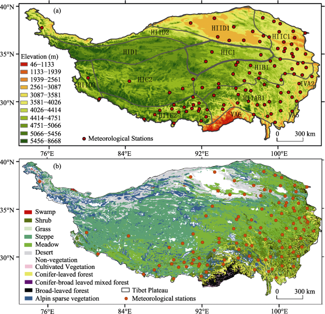
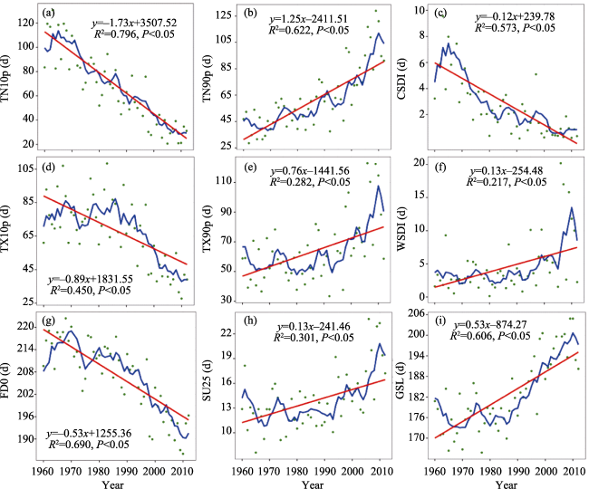
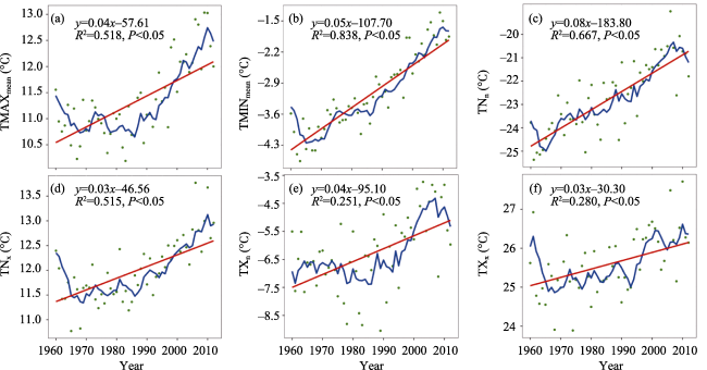
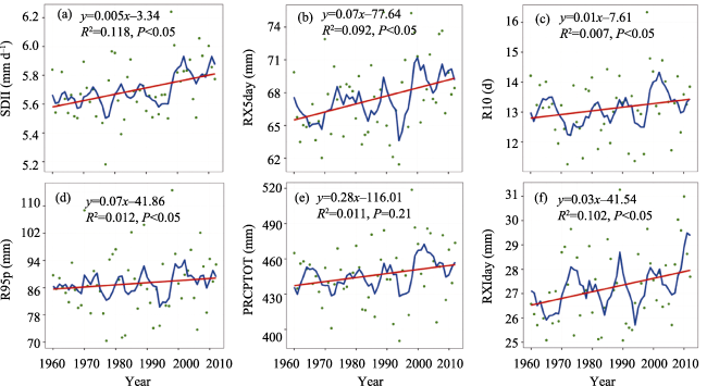
Extreme climate events play an important role in studies of long-term climate change. As the Earth’s Third Pole, the Tibetan Plateau (TP) is sensitive to climate change and variation. In this study on the TP, the spatiotemporal changes in climate extreme indices (CEIs) are analyzed based on daily maximum and minimum surface air temperatures and precipitation at 98 meteorological stations, most with elevations of at least 4000 m above sea level, during 1960-2012. Fifteen temperature extreme indices (TEIs) and eight precipitation extreme indices (PEIs) were calculated. Then, their long-term change patterns, from spatial and temporal perspectives, were determined at regional, eco-regional and station levels. The entire TP region exhibits a significant warming trend, as reflected by the TEIs. The regional cold days and nights show decreasing trends at rates of -8.9 d (10 yr)-1 (days per decade) and -17.3 d (10 yr)-1, respectively. The corresponding warm days and nights have increased by 7.6 d (10 yr)-1 and 12.5 d (10 yr)-1, respectively. At the station level, the majority of stations indicate statistically significant trends for all TEIs, but they show spatial heterogeneity. The eco-regional TEIs show patterns that are consistent with the entire TP. The growing season has become longer at a rate of 5.3 d (10 yr)-1. The abrupt change points for CEIs were examined, and they were mainly distributed during the 1980s and 1990s. The PEIs on the TP exhibit clear fluctuations and increasing trends with small magnitudes. The annual total precipitation has increased by 2.8 mm (10 yr)-1 (not statistically significant). Most of the CEIs will maintain a persistent trend, as indicated by their Hurst exponents. The developing trends of the CEIs do not show a corresponding change with increasing altitude. In general, the warming trends demonstrate an asymmetric pattern reflected by the rapid increase in the warming trends of the cold TEIs, which are of greater magnitudes than those of the warm TEIs. This finding indicates a positive shift in the distribution of the daily minimum temperatures throughout the TP. Most of the PEIs show weak increasing trends, which are not statistically significant. This work aims to delineate a comprehensive picture of the extreme climate conditions over the TP that can enhance our understanding of its changing climate.

Cite this article

ZHOU Yuke . Characterizing the Spatio-temporal Dynamics and Variability in Climate Extremes over the Tibetan Plateau during 1960-2012[J]. Journal of Resources and Ecology, 2019 , 10(4) : 397 -414 . DOI: 10.5814/j.issn.1674-764X.2019.04.007

1 Introduction

In global change studies, most analyses have used observational temperature and precipitation data, and have focused on changes in mean values. Compared with gradual changes in mean climatic factors, extreme weather or climate events have a greater potential for disastrous impacts to society and the environment. Climate change is mainly driven by external factors, such as the increase in the global atmospheric concentrations of greenhouse gases, or other human activities (Adger et al., 2009; Stocker et al., 2013; Katz et al., 1992). With the availability of daily maximum and minimum records, analyzing changes in extreme climate events, such as heat waves and extreme rainfall, can allow the detection of climate changes at a fine temporal resolution. Studies based on the NOAA Storm Events Database and public opinion data demonstrate that recent extreme weather activities can reflect the changing climatic conditions (Konisky et al., 2016), such as temperature extremes, precipitation extremes, tropical storms, and hydrological extremes (Zwiers et al., 2013; Alexander et al., 2006; Brunner et al., 2017). These extreme events have a strong impact on the local ecological conditions and human lives (Ummenhofer et al., 2017; Herold et al., 2017). To better describe the extreme climate events, the joint World Meteorological Organization Commission for Climatology (CCl)/World Climate Research Program (WCRP) project of the Climate Variability and Predictability (CLIVAR) Expert Team have defined a suite of climate extreme indices (CEIs). These indices enable global change analysis based on temperature and precipitation extremes. Previous studies using temperature indices have shown that these indices can reflect the warming trend of climate change (Alexander et al., 2006). Dong et al. (2017) have examined the contribution of temperature extremes to shaping the mean surface air temperature and found a rapid increase in the daily maximum temperature during summer over Western Europe. Tao et al. (2017) revealed that the minimum and maximum temperatures have different impacts on the growth of winter wheat. The decreases in the cold indices and increasing rainfall are widely reported in the literature from various countries (Xiao et al., 2016; Tangang et al., 2017).
The Tibetan Plateau (TP) is a unique geomorphic region composed of specific geomorphic types, such as extreme high mountains, plains, and plateaus of either high or sub- high altitudes. TP has an average altitude of over 4000 m above sea level and an area of 2.5 million square kilometers (Zhang et al., 2002). It has been a popular study area because of its sensitivity to the ongoing global climate change. A number of studies have focused on its changing climate based on either station-observed meteorological data or remotely sensed data from across the TP (Lu et al., 2015; Duan et al., 2015; Guo et al., 2012; An et al., 2016; Shen et al., 2015; Luo et al., 2016). According to previous studies, the TP has undergone a significant warming trend in the last few decades (approximately 0.16℃ (10 yr)-1 for the annual mean during the period 1955-1996) (Liu et al., 2006; Lin et al., 1996; Piao et al., 2016), while wind speed and solar radiation have declined over the last three decades (Yang et al., 2011). The TP began warming earlier than the Northern Hemisphere and the global average, which may reflect its heightened sensitivity to global change (Liu et al., 2000). It has been documented that the precipitation is increasing in the eastern and western TP and decreasing in the middle area (Lu et al., 2015). In addition, the precipitation has a heterogeneous spatial pattern because of the large-scale atmospheric circulation and temperature changes.
Over the past decade, many studies have focused on changes in the overall temperature or precipitation based on their mean values, and only a few studies have explored the extreme climate events on the TP. Using the CEIs derived from daily data, the asymmetry in climate change can be examined, especially the seasonal and diurnal heterogeneous warming (Tan et al., 2015; Shen et al., 2016). The daily minimum temperature was found to have strong impacts on the spring phenology of vegetation on the TP (Shen et al., 2016). Several studies have indicated an asymmetric pattern of warming trends in nighttime temperatures that are larger than those in daytime temperatures (Liu et al., 2006; Jun, 2001). It has been reported that in strong warming periods, the change in the mean temperature still has a dominant effect on extreme temperature events (Song et al., 2014). The daily precipitation has increased substantially, while the cool indicators have decreased within China (Xiao et al., 2016). Due to inadequate long-term data and the complex ecosystem of the TP, climatic changes, especially changes in the extreme events, remain unclear and uncertain. Thus, further studies should be performed on the climatic extremes on the TP.
Knowledge of the climatic extremes on the TP has been inadequate for a long time, due to the lack of sufficient observational data. However, with the current availability of long-term ground observation datasets, spatiotemporal trends and variability of the temperature and precipitation extremes can be assessed for the period of 1960-2012. Besides monotonic trend analyses, abruptly changing conditions of climate extremes, as well as topographical impact factors, are examined in this study. Through a comprehensive and detailed exploratory analysis, climate extreme conditions are clearly depicted.

2 Materials and methods

2.1 Study area and meteorological data

The daily meteorological dataset used in this study was obtained from the National Climate Center, China Meteorological Administration (CMA), and it includes data from 98 stations throughout the TP. The spatial distribution of these meteorological stations is shown in Fig. 1. In the early years, the meteorological data from these stations were collected using manual observations, and subsequently, the data have been progressively obtained using automatic observation equipment. The National Climate Center has processed the dataset from different observation methods to maintain their consistency (China Meteorological Administration, 2003). The dataset for this study was produced with primary data quality control following the Chinese surface weather observation and statistical standards (China Meteorological Administration, 2003; China Meteorological Administration, 2005). Following these standards, the homogenization of the data has been checked, and other studies from the CMA have demonstrated the process of homogenizing the same dataset Li et al., 2009 (Li et al., 2010; Li et al., 2017). For the non-homogenized data, data processing is perfor-med according to the conditions that led to the non-homogenization of the data. In some cases, the position of the weather station changed. If there are significant differences in the terrain conditions between the old station and new station, if the distance between them is greater than 100 km, or if the elevation difference is more than 100 m, then the records from the station with the longest observation history are included in the final CMA Meteorological dataset. If the observed records in the old and new stations have the same historical time length, then the newer records are selected. In other cases, if the observation instruments had changed, then the observed records are corrected according to the instrument errors. In this study, data quality was also checked to ensure data integrity and continuity within the time series. Obvious errors in the observation records are excluded, such as: 1) daily minimum values that are larger than the daily maximum values, 2) precipitation below zero, and 3) records that are more than three times the standard deviation of the station records. The missing values in the temperature and precipitation time series are assigned values of -99.9, which can be recognized by the R package RclimDex (Zhang et al., 2004). The raw temperature dataset was multiplied by a scale factor of 0.1 to obtain the real values of the observed temperatures. Further data processing was performed automatically by RClimDex. The typically observed meteorological factors, including daily precipitation, daily maximum temperature and daily minimum temperature, are chosen for computing the climate extreme indices during the period of 1960-2012.
Fig. 1 Maps showing the terrain (a) and land cover (b) on the TP. Red points represent the 98 meteorological stations in the study area
These stations span three temperature zones, consisting of 10 eco-geographical regions (ecoregions) (Wu et al., 2003). They are located in (1) the plateau temperate zone (HIIAB1, HIIC1, HIIC2, HIID1, HIID2 and HIID3), (2) the plateau sub-frigid zone (HIB1, HIC1, HIC2 and HID1), and (3) the middle subtropical zone (Fig. 1a). The detailed interpretations of the 10 ecoregions are provided in Table 1. Due to the complex natural conditions, there are fewer stations in the northwestern TP. These stations are all located above 2000 m a.s.l. on the TP and most of the records date from the mid-1950s onward.
Table 1 Codes and interpretations for the seven eco- geographical regions
Region Code Interpretation
HIIAB Temperate, humid or semi-humid zone
HIIC Temperate, semi-arid zone
HIID Temperate, arid zone
HIB Sub frigid, semi-humid zone
HIC Sub frigid, semi-arid zone
HID Frigid, arid zone
VA Mid subtropical, humid zone
The land cover types (Liu et al., 2003) of these meteorological stations are shown in Fig. 1b. A large percentage of the stations are located in grassland (approximately 42%, including steppe and meadow), followed by 23% in cropland, 16% in shrubland, 10% in forest, and 9% in bare land or desert.

2.2 Climate extreme indices

A suite of CEIs, which was proposed by the World Meteorological Organization (WMO), was calculated in this study based on the daily meteorological data from the 98 stations on the TP. We selected 15 temperature extreme indices (TEIs) and 8 precipitation extreme indices (PEIs) to explore trends and changing patterns of the extreme climatic events during 1960-2012 (Table 2). After preprocessing and quality control of the raw meteorological data, the R package RClimDex was used to compute the CEIs (Zhang et al., 2004).
Table 2 Definitions of the climate extreme indices (CEIs)
Name* Descriptive name Definition Units
TN10p Cold nights Percentage of days when TN < 10th percentile d
TN90p Warm nights Percentage of days when TN > 90th percentile d
TX10p Cold days Percentage of days when TX < 10th percentile d
TX90p Warm days Percentage of days when TX > 90th percentile d
CSDI Cold spell duration indicator Annual count of days with at least 6 consecutive days when TN < 10th percentile d
WSDI Warm spell duration indicator Annual count of days with at least 6 consecutive days when TX > 90th percentile d
FD0 Frost days Annual count of days when TN < 0℃ d
ID0 Ice days Annual count of days when TX < 0℃ d
SU25 Summer days Annual count of days when TX (daily maximum) > 25℃ d
GSL Growing season Length Annual (1st Jan to 31st Dec in NH, 1st July to 30th June in SH) count between first span of at least 6 days with mean temperature > 5℃ and first span after July 1 (January 1 in SH) of 6 days with mean temperature < 5℃ d
TNn Min Tmin Monthly minimum value of daily minimum temp
TNx Max Tmin Monthly maximum value of daily minimum temp
TXn Min Tmax Monthly minimum value of daily maximum temp
TXx Max Tmax Monthly maximum value of daily maximum temp
TMAXmean Mean of maximum value of daily average temperature
TMINmean Mean of minimum value of daily average temperature
SDII Simple daily intensity index Annual total precipitation divided by the number of wet days (defined as PRCP ≥ 1.0 mm) in the year Mm d‒1
R10p Number of heavy precipitation days Annual count of days when precipitation ≥10 mm d
CWD Consecutive wet days The longest span of consecutive days when daily precipitation < 1mm d
CDD Consecutive dry days The longest span of consecutive days when daily precipitation > 1mm d
R95p Very wet days Annual total precipitation when precipitation > 95th percentile mm
RX5day Max 5-day precipitation amount Monthly maximum precipitation for a continuous 5d span mm
RX1day Max 1-day precipitation amount Monthly maximum 1-day precipitation mm
PRCPTOT Annual total wet-day precipitation Annual total precipitation in wet days (precipitation ≥ 1mm) mm

Note: *TX means daily maximum temperature; TN means daily minimum temperature.

2.3 Methods

2.3.1 Trend and persistence analysis
A simple linear regression model was applied to estimate the long-term trends of each climate extreme index time series at multiple scales. Each climate index was regressed with the corresponding years (1960-2012) as the equation${{y}_{i}}=a\times {{t}_{i}}+b~\ (i=1,2,\cdots ,n)$, in which y represents one index, t represents the year in which it occurred, n is the sample size, and a and b are the linear regression coefficient and constant term, respectively, which can be calculated by the least squares method (see Equations (1) and (2)). The significance of the linear fitting results is tested using Student's t-test. The linear fitting is also estimated using Theil-Sen trend analysis and the Mann-Kendall test, which have various modifications (Tegos et al., 2017).
$a=\frac{~\sum\limits_{i=1}^{n}{{{y}_{i}}\times t}-~\frac{1}{n}\left( \sum\limits_{i=1}^{n}{{{y}_{i}}} \right)\times \left( \sum\limits_{i=1}^{n}{{{t}_{i}}} \right)}{\sum\limits_{i=1}^{n}{t_{i}^{2}}-~\frac{1}{n}{{\left( \sum\limits_{i=1}^{n}{{{t}_{i}}} \right)}^{2}}}~,\begin{matrix} {}&{} \\\end{matrix}b=\bar{y}-a\bar{t}$(1)
where
$\bar{y}=~\frac{1}{n}\underset{i=1}{\overset{n}{\mathop \sum }}\,{{y}_{i}},\ \begin{matrix} {}&{} \\\end{matrix}\bar{t}=\frac{1}{n}\underset{i=1}{\overset{n}{\mathop \sum }}\,{{t}_{i}}$ (2)
The Hurst exponent is widely used in the fields of hydrological science and climate change, where it plays an important role in predicting the persistence of time series data (Hurst, 1951; Weron, 2002; O’Connell et al., 2016). Here, we applied this method to detect the future tendency of each CEI’s time series. Specifically, the reliable R/S method-based Hurst exponent is selected according to previous studies (Weron, 2002). R/S analysis is used to estimate the auto-correlation properties of a time series. A time series of full-length N is divided into a number of shorter time series of lengths n = N, N/2, N/4, and so on. The average rescaled range is then calculated for each value of n as follows:
1) As X = X1, X2,…, Xn, calculate the mean value m,
$m=\text{ }\!\!~\!\!\text{ }\frac{1}{n}\text{ }\!\!~\!\!\text{ }\underset{i=1}{\overset{n}{\mathop \sum }}\,{{X}_{i}}$(3)
2) Derive a new time series adjusted by m,
Yt = Xt - m, t = 1, 2,…, n (4)
3) Calculate the cumulative deviation series Z,
${{Z}_{t}}=\text{ }\!\!~\!\!\text{ }\!\!~\!\!\text{ }\underset{i=1}{\overset{t}{\mathop \sum }}\,{{Y}_{i}}$ (5)
4) Calculate the range R,
R(n) = max(Z1, Z2,…, Zn) - min(Z1, Z2, …, Zn) (6)
5) Calculate the standard deviation S,
$S\left( n \right)=\text{ }\!\!~\!\!\text{ }\!\!~\!\!\text{ }\sqrt{\frac{1}{n}\underset{i=1}{\overset{n}{\mathop \sum }}\,{{\left( {{X}_{i}}-m \right)}^{2}}}$ (7)
6) Calculate the rescaled range R(n)/S(n) and average over all the partial time series of length n. The H value is derived by fitting the following formula:
$\frac{R\left( n \right)}{S\left( n \right)}=C\times {{n}^{H}}$ (8)
The Hurst exponent (H) values range from 0 to 1, and this range can be divided into two parts by 0.5. H = 0.5 indicates a random series. When 0.5 < H < 1.0, the long-term autocorrelation of the time series is persistent, and the persistence will become stronger as H becomes closer to 1.0. In other words, a persistent time series means the direction of the next value is more likely to be the same as the current value. The larger the H value, the stronger the trend. In contrast, a value of H in the range of 0-0.5 means that the long-term autocorrelation of the time series is anti-persistent; and the closer the H value is to 0.0, the stronger the anti-persistence. According to previous experiments on the application of the Hurst exponent, a Hurst exponent close to 0.5 indicates a random walk time series, meaning that there is no relationship between the observed values and the forecasted values in the future. Thus, an anti-persistent series has a characteristic of “mean-reverting”, which means an “up” value is more likely to be followed by a “down” value, and vice versa.
2.3.2 Variability and change point analysis of the time series
In probability theory and statistics, the coefficient of variation (CV) is a standardized measure of dispersion that is often expressed as a percentage. The actual value of the CV is independent of the units in which the measurement has been taken, so it is useful when making comparisons between data sets with different units. Here, CV is applied to detect the inter-annual variability of the CEIs time series. The CV is calculated by the following formula (Equation 3).
$CV=~\frac{1}{n}\sqrt{\frac{\sum\limits_{i=1}^{n}{{{\left( {{x}_{i}}-\bar{x} \right)}^{2}}}}{n-1}}\times 100%$(9)
where xi is one climate extreme index in the ith year, and $\bar{x}$ is the corresponding mean value during n years (here, 1960-2012). A larger value of CV represents a more significant fluctuation in the extreme index time series, while a smaller value is indicative of a time series that is more stationary.
For a yearly time series, a change point refers to a year in which a shift occurs. In general, there are many methods for obtaining the change point in a time series, such as the F-test, Pettitt test, Mann-Kendall test and so on. Since the ECI time series is used to show a tendency in the long-term period, the nonparametric Pettitt test method is adopted to find the shift year, before and after which the average values of the parts of the time series indicate a pronounced difference. In the Pettitt test, the null hypothesis, H0, is that the data in the time series are independent and randomly distributed, while the alternative hypothesis, H1, is that there is a time point t dividing the time series into two parts that follow different distributions. The detailed supporting information about the utility of the Pettitt test is referenced in a previous study (Pettitt, 1979). We carried out the following steps to detect change points in the time series of the CEIs:
1) Rank the annual CEI data (X) from 1 to N (i.e., X1, X2,…, Xn).
2) Calculate the value of Vi:
Vi = N + 1–2Ri, i = 1, 2,…, N (10)
where Ri is the rank of Xi in the CEI time series.
3) Calculate the value of Ui:
Ui = Ui-1 + Vi (11)
U1 = V1 (12)
4) Determine the most likely change point, which occurs at the ith observation when
KN = max1< i < N|Ui| (13)
5) Estimate the critical value of Poa
${{P}_{oa}}=2{{\text{e}}^{-\frac{6{{K}_{N}}^{2}}{\left( {{N}^{3}}+{{N}^{2}} \right)}}}$(14)
If Poa< α, where α is the statistical significance of the test, then the null hypothesis is rejected. In this study, α is set as 0.05. After passing the significance test, the change point year is determined.
2.3.3 Stepwise regression between observed values and CEIs
Given the variety of CEIs in this study, it is important to estimate their contributions to the normal climatic conditions. We mainly use the stepwise regression technique to determine which CEIs variables have a greater impact on the observed meteorological values of TMINmean, TMAXmean and PRCTOT. In addition, the growing season length (GSL) index is involved in this step. The stepwise regression approach is an iterative regression process to select the most important independent variables. Usually, there are two stepwise regression methods. One is based on the forward addition of variables, and the other is accomplished through the backward subtraction of variables from the set of explanatory variables. In our study, the backward stepwise regression is applied and the final explanatory variables are selected based on the AIC (Akaike Information Criterion) statistics.

3 Results

3.1 Trend analysis at the regional scale

On the TP regional scale, the long-term trends of the temperature and precipitation indices are demonstrated in this section. The CEIs for the entire TP region were calculated as the average values of the index values from all stations. The CEIs time series were first smoothed with a 5-year window width, and then fitted with the linear regression model (see the Methods section).
3.1.1 Temperature extreme indices
Fig. 2 shows the temporal evolution of the temperature extreme indices and trends on the TP. The original indices present significant dispersion patterns in the time series. According to the definitions, these TEIs could be classified into two main types that consist of warm indices and cold indices. The growing season length (GSL) is derived from the daily temperature evolution, so it can be used as an indicator of changing temperature conditions. As indicated by the red lines in Fig. 2, it is quite obvious that the warm indices (TN90p, TX90p, WSDI, SU25) and the GSL have displayed increasing tendencies since the 1960s, while the slopes of the cold indices (TN10p, CSDI, TX10p, FD0) have decreased over the years. Specifically, with respect to the cold indices, the cold night indicator (TN10p) shows the fastest decline with a speed of 17.3 d (10 yr)‒1 (days per decade), followed by the cold days (TX10p), the frost days indicator (FD0) and the cold spell duration indicator (CSDI), with the slopes of the trends at -8.9 d (10 yr)‒1, -5.3 d (10 yr)‒1 and -1.2 d (10 yr)‒1, respectively. For the warm indices, all of them show increasing trends. Among them, the indicator with the fastest increase is the warm night indicator (TN90p), which has increased by 12.5 d (10 yr)‒1. The warm days indicator (TX90p), summer days indicator (SU25) and warm spell duration indicator (WSDI) have rates of change of 7.6 d (10 yr)‒1, 1.3 d (10 yr)‒1 and 1.3 d (10 yr)‒1, respectively. From the above results, the rates of increase in the warm indices are slower than the rates of decrease in the cold indices, which to some extent reflects the asymmetry of the changing trends of the cold and warm indices over the last 53 years. The GSL has been extended by 5.3 d (10 yr)‒1 for the period of 1960-2012. Generally, compared with the warm indices, the cold indices demonstrate larger changes as reflected by the absolute values of the linear fitting slopes. Several comparisons can be made between the change rates, such as TN10p 17.3 d (10 yr)‒1 versus TN90p 12.5 d (10 yr)‒1, or TX10p 8.9 d (10 yr)‒1 versus TX90p 7.6 d (10 yr)‒1. In other words, these comparisons reflect the asymmetry of the changing trends of the cold and warm indices over the past 53 years, but both indices are developing toward a warming condition.
To further assess the trends of the TEIs, we applied the Theil-Sen slope detection method, as well as the MK-test, on the time series (Table 3). The Theil-Sen slopes of these indices are consistent with the slopes derived from the linear fitting model. Specifically, the magnitudes of the Theil-Sen slopes are approximately equal to the linear values. For instance, TN10p is -1.73 vs. -1.726, FD0 is -0.53 vs. -0.504, and GSL is 0.53 vs. 0.528 when comparing the linear fitting model slopes and the Theil-Sen slopes, respectively. For the measure of Kendall’s tau, which is the output of the MK-test, a negative value indicates a decreasing trend for a time series, while a positive value represents an increasing trend. Its absolute value indicates the magnitude of the trend. For the temperature extreme indices, these Kendall’s tau values have the same developing directions (negative or positive) as the linear regression and Theil-Sen slopes. In addition, the absolute values of the Kendall’s tau values mostly keep the same ranks as the other two methods. In Table 3, all the scores pass the test of significance using the MK-test (Hamed, 2008) at the 1% level.
Table 3 Theil-Sen trends and MK-test values for temperature extreme indices
Trend\Indices TN10p TN90p CSDI TX10p TX90p WSDI FD0 SU25 GSL
Theil-Sen Slope -1.726** 1.025** -0.108** -0.800** 0.568** 0.080** -0.504** 0.093** 0.528**
Kendall’s tau -0.885** 0.749** -0.762** -0.562** 0.443** 0.478** -0.702** 0.457** 0.636**
Trend\Indices ID TMAXmean TMINmean TNn TNx TXn TXx
Theil-Sen Slope -0.334** 0.031** 0.051** 0.079** 0.027** 0.043** 0.027**
Kendall’s tau -0.655** 0.508** 0.811** 0.852** 0.61** 0.473** 0.493**

**: P < 0.01

Fig. 2 Temporal evolution of the TEIs and trends on the TP (green points represent original index values; blue lines are 5-year smoothing averages; red lines are the linear fitting lines).
In addition to the above indices, the temporal evolution of the observed temperature extreme values, including TMAXmean, TMINmean, TNn, TNx, TXn, and TXx, is characterized at the scale of the entire TP (Fig. 3). All these values illustrate increasing trends that are statistically significant. The minimum value of the daily minimum temperature indicator (TNn) has increased by approximately 5℃ since 1960. The corresponding maximum value of the daily maximum temperature indicator (TXx) has only increased by approximately 1.5℃ over the 53 years. TXn and TNx have increased by approximately 3℃ and 2℃, respectively, during 1960-2012. In addition, the minimum value of the daily average temperature indicator (TMINmean) increased slightly faster than the maximum value of the daily average temperature indicator (TMAXmean), namely 0.5℃ (10 yr)-1 vs. 0.4℃ (10 yr)-1, respectively, which also reflects the asymmetry of the warming trend among the different temperature indicators. What this means is that the temperature increase on the coldest night is the largest, while that during the day is the smallest. Each of the linear fittings in Fig. 3 pass the significance test at the 0.05 level. In the time span of 1980-1990, there is an apparent decrease in the fluctuation of the time series of TMAXmean, TNx, and TXn. According to the Theil-Sen slopes and MK-test values (Table 3), the minimum temperature extremes have a larger increasing trend than the maximum temperature extremes. For instance, the slope of TMAXmean is 0.031, which is smaller than that of TMINmean at 0.051. As time has passed, the minimum value of the daily minimum temperature (TNn) has increased faster than the maximum value of the daily minimum temperature (TNn of 0.079 vs. TNx of 0.027). The daily maximum temperature indices have the same relation, where TXn is 0.043 and TXx is 0.027.
Fig. 3 Temporal evolution of maximum and minimum observed temperature on the TP (green points represent original index values; blue lines are 5-year smoothing averages; red lines are the linear fitting lines)
From observations of the overall trends of the TEIs, the entire TP has become significantly warmer during the study period, with the temperature increasing by an average of 3℃. This phenomenon is in agreement with the global warming tendency. However, the warming trend in the TP shows asymmetry, which is reflected by three aspects: 1) The decreasing rate of the cold nights indicator (TN10p) is 8.4 d (10 yr)-1; which is greater than that of the cold days indicator (TX10p), showing the more pronounced difference than other indices, while the increasing rate of the warm nights indicator (TN90p) is 4.9 d (10 yr)-1, which is greater than that of the warm days indicator (TX90p). 2) The decreasing rate of the cold indices is faster than the increasing rate of the warm indices, such as the increase of 17.3 d (10 yr)-1 for the cold nights indicator (TN10p), compared to the decrease of the warm nights indicator (TN90p) by 12.5 d (10 yr)-1. 3) The minimum value of the temperature extreme indices increased slightly faster than the maximum value of the TEIs.
3.1.2 Precipitation extreme indices
Similar to TEIs, the time series and linear fitting results of PEIs are depicted in Fig. 4. The PEIs consist of (a) simple daily intensity index (SDII), (b) maximum precipitation for a continuous 5d span (RX5day), (c) days of precipitation ≥10 mm (R10), (d) very wet days (R95p), (e) total annual precipitation (PRCPTOT), and (f) maximum precipitation for a continuous 1d (RX1day)).
Fig. 4 Temporal evolution of precipitation extreme indices (PEIs) on TP (green points represents original index values; blue lines are 5-year smoothing averages; red lines are the linear fitting lines)
It should be noted that, except for PRCTOT, the trends of the other precipitation indicators are significant at the 95% level. In contrast to the TEIs, the significance of the changes in PEIs is low, which may be caused by the low rainfall in the middle and western TP. In addition, the fluctuations in the time series of the PEIs are more pronounced compared with the TEIs. Besides the low rainfall level, these variations may also be attributed to the relatively uniform distribution of precipitation over time. For example, according to the raw data in this study and a previous study (Zhang et al., 2015), precipitation on the TP is mainly concentrated in summer. Annual PEIs calculated from daily rainfall data will span a wide range of values. The regional occurrence of R10 has increased by 0.1d (10 yr)-1, while the occurrence of extreme precipitation >95% and five days’ maximum precipitation both have increased by 0.7 mm (10 yr)-1. The Theil-Sen trend test results also indicate the lower developing trend of PEIs (Table 4).
Table 4 Theil-Sen trend and MK-test for PEIs
Trend\Indices SDII RX5day R10 R95p PRCPTOT RX1day CDD CWD
Theil-Sen Slope 0.004** 0.071** 0.011* 0.060* 0.079* 0.057* -0.310** -0.002
Kendall’s tau 0.406** 0.434** 0.235* 0.202* 0.302* 0.410* -0.419** -0.087

*: P < 0.05, **: P < 0.01

3.2 Trend analysis at the eco-geographical regional and station scales

To obtain more information about CEIs changes at smaller scales, an eco-geographical region study is conducted to determine the spatial pattern of the CEIs distribution. The definitions of eco-geographical regions on the TP include not only the characteristics of climatic and geographical factors, but also involve vegetation information (Stocker et al., 2013). In addition, the climate and vegetation in each ecoregion show good uniformity. Therefore, the study of climate change trends for ecoregions can better reveal the characteristics of regional differences on the plateau.
The CEIs for each ecoregion were computed as the averages of CEIs for the stations within it. The long-term trend of the regional CEIs time series is fitted with the linear regression method. A thematic map shows the slope of the trend for each extreme index (Fig. 5). From this map, we can see that the negative or positive slope patterns between the indices in different ecoregions are consistent, but the ranges of the slope values vary between different regions. HIID1 is the most significant ecoregion, in which the slope value is larger than those in the other regions. In particular, the absolute values of Tn10p, TN90p, TX10p, TX90p, and RX1day in these ecoregions are almost all the largest.
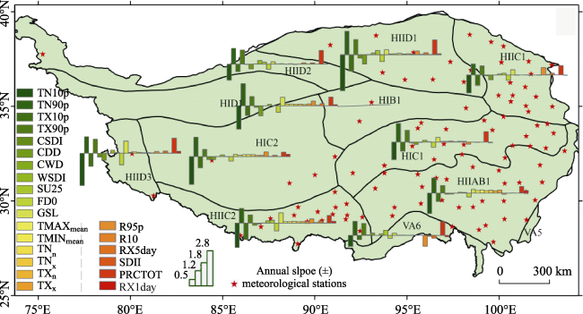
Fig. 5 Slopes of long-term trends for the CEI at the eco-geographical region scale (bar height indicates slope, upward bars denote positive slopes and downward bars are negative slopes)
At the regional scale, the TEIs have significant change trends during the period of 1960-2012. In most of the regions, the cold indices (such as TN10p and TX10p) in TEIs present decreasing trends as indicated by the negative slopes, while the warm indices (such as TN90p and TX90p) show increasing trends. This phenomenon also exists at the station scale and the scale of the entire TP. Except for PRCTOT, none of the other PEIs show a substantial trend in the eco-geographical regions. The trend for PRCTOT means that the annual total precipitation on wet days has an increasing trend in the northern arid area (HIID) and southern humid area (VA6).
At the station level, most of the TEIs show statistically significant changing trends (green triangles in Fig. 6). TN10p, TX10p, CSDI and FD0 for each station displays a negatively changing slope, while TN90p, TX90p, WSDI and GSL have positively increasing trends. These results are consistent with the findings at the eco-geographical region scale. Except for TX10p, the trends of the other indices for the eastern and middle stations do not display a pronounced difference; in other words, we do not find a regular pattern in the spatial distribution of the TEIs changing trends. The changing magnitudes of WSDI, FD0, and GSL are relatively small compared those of TN10p, TX10p, TN90p, and TX90p, which are either cold or warm extreme indices. From the spatial pattern, we find the magnitudes of the trends of TN10p, TX10p, TN90p and TX90p in the northern TP, mainly in the HIID1 ecoregion, are more significant than those in the other parts of the TP.
The trends at the station level showed high-spatial heterogeneity, as indicated in Fig. 7. Compared with the TEIs, typical PEIs at most of the stations do not show statistically significant trends. For example, only some stations in the northeastern arid area have a spatial cluster pattern of significant SDII trends, but a considerable number of the stations do not pass the significance test at the 0.05 level. For RX5day, R10, and R95p, the changing magnitudes are small, and some stations’ trends are not significant.
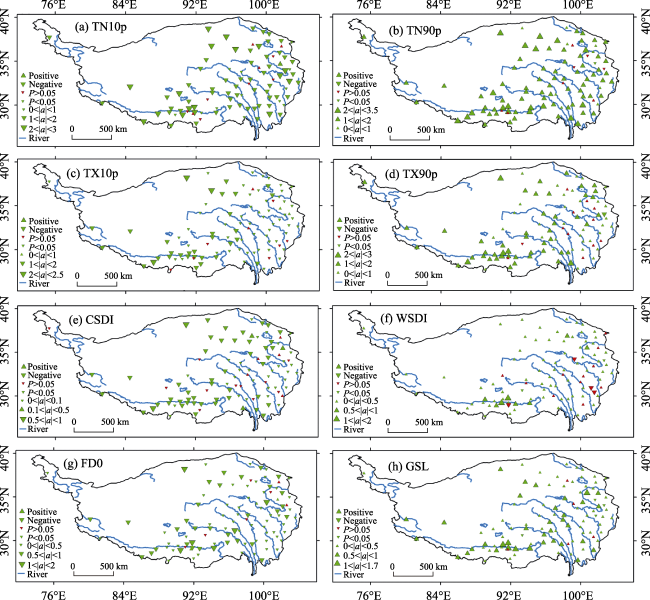
Fig. 6 Trends of the typical TEIs at the station scale. Upward and downward triangles, respectively, represent positive and negative trends for TEIs. |a| is the absolute magnitude of a trend.
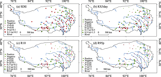
Fig. 7 Same as Fig. 6, but for typical PEIs

3.3 Probability distribution of the time series change points

For each extreme index, we calculated the probability density distribution of the change points in its time series among the 98 stations (Fig. 8). We found that each of the probability density distribution conditions presents a bell curve shape. The peaks of almost all the curves appear in the time period of 1980-2000 (around the year 1990). The change point of CSDI occurs in the earlier 1980s. This finding suggests that the climatic conditions over the Tibetan Plateau changed significantly in the 1990s.
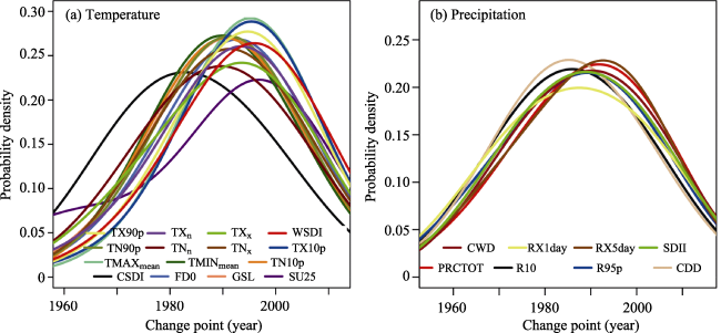
Fig. 8 Probability density distribution of change points for CEIs at the 98 stations

3.4 Relationship between climate extreme indices and elevation

For these 98 stations, we analyzed the distribution of the linear slopes of the CEI with elevation using a violin plot, which combines a boxplot and a kernel density plot (Fig. 9). For each CEI linear slope, the altitude range is split into equal intervals of 500 m. The statistical distribution condition of the linear trends of the stations in one interval (i.e., stations at a 500 m elevation interval) is drawn on one violin plot. The black box indicates the interquartile range and the white point is a marker for the median of the data. According to the median slopes (the white dots in the figure), most of the linear slopes of the TEIs do not change significantly with increasing elevation. However, there is a slight upward trend for the TN90p median slopes at elevations above 3 km, and the median slopes of SU25 decrease as elevation increases.
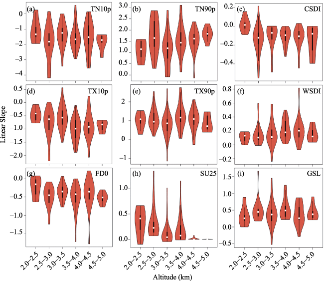
Fig. 9 Violin plots demonstrating the distribution of TEIs linear slopes at various elevation intervals (500 m is the interval, temporal regression slopes of the sites in each interval comprise a violin plot)
In Fig. 10, the median linear slope of the four precipitation indices has only a minimal response to the variation in elevation. The median of the linear slopes also illustrates the lower magnitude of the changing trend in PEIs. For a considerable number of stations, the PEIs linear slopes shownegative trends.
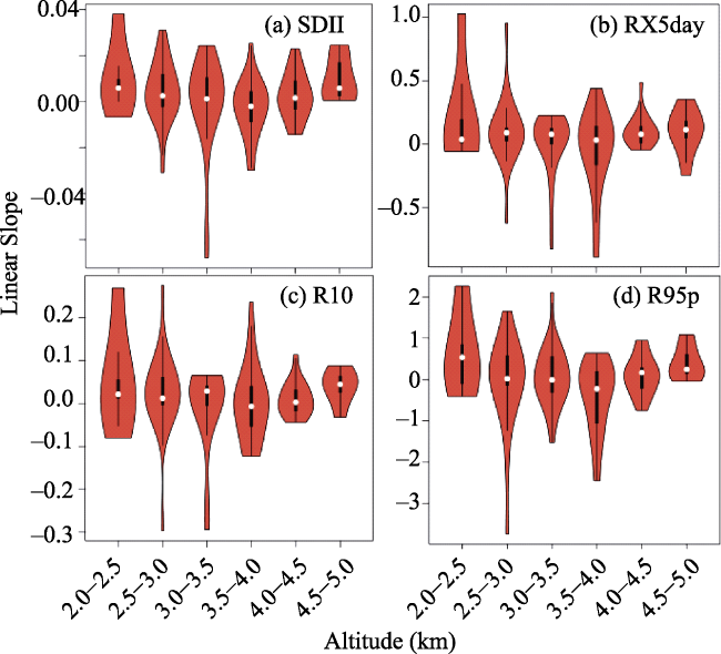
Fig. 10 Same as Fig.9 but for PEI

3.5 Persistence of climate extremes

According to the R/S method (Weron, 2002), the Hurst exponents were calculated for various CEI time series (Fig. 11). The black dotted line indicates the position of 0.5.
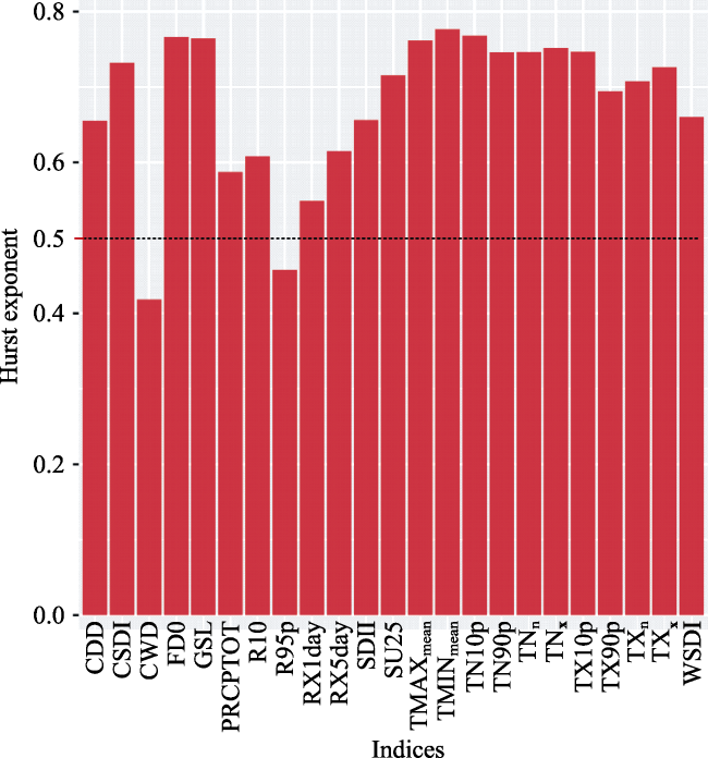
Fig. 11 The Hurst exponents of the climate extreme indices
Most of the Hurst exponents are above the level of 0.5, indicating that the time series of these indices will maintain a persistent trend in the future (Fig. 11). However, there are some indices for which the Hurst exponent values are relatively close to 0.5. By careful observation, we can see that most of them are precipitation indices, such as CWD, PRCPTOT, R95p, and RX1day. This finding indicates that the precipitation extremes on the TP are not very predictable. The lower slopes of the linear trends for these PEIs in Fig. 4 also confirm this result. Meanwhile, the temperature extreme indices have relatively higher Hurst exponents. Among them, the persistence of the FD0, GSL, TMAXmean, TMINmean and TN10p indices are stronger because their Hurst exponents are close to one.

4 Discussion

As the Third Pole of the Earth, the TP is sensitive to global climate change. Studying the climate extremes over the TP is useful for enhancing our understanding of its climatic patterns. In this study, the TEIs, either at the regional or station levels, delineate a significant warming trend for the TP. However, a pronounced asymmetric pattern shows that the warming trend in cold indices is greater than that in warm indices. This finding on the TP is consistent with similar results from a global scale study that show the Earth’s temperature is increasing more rapidly at night than during the day (Flato et al., 2013). Other published studies also demonstrate that the TP has experienced a pronounced warming over the past decades (Duan et al., 2015; Zhang et al., 2013). The spatially heterogeneous warming rate, which is inferred from TEIs in this study, has also been reported previously (Duan et al., 2015). Studies on vegetation and its corresponding phenology have also demonstrated that vegetation has a positive response to the warming of the TP, through the greening of vegetation and advanced dates of spring phenological events (Zhu et al., 2016; Yang et al., 2017). The sustainably changing trends in most of the TEIs, indicated by the Hurst exponents, are not surprising within the context of continued warming of the Northern Hemisphere. As the TP is mostly covered by arid and semiarid areas, the development of precipitation indices that are non-significant may be attributed to the natural climate variability. It has been demonstrated that precipitation on the central TP shows an increasing trend, but on the south and the east Plateau, it shows a decreasing trend, while the western part has only a small amount of precipitation (Yang et al., 2014). This spatial heterogeneity in precipitation may lead to the insignificance of the developing trends of PEI for the entire TP area in our study period of 1960-2012.
The ability to discover abrupt breaking points using CEIs is useful for monitoring climatic disturbances. The turning points found in the CEIs time series in this study are mostly distributed in the period of 1980-1990. This phenomenon may provide evidence of the climate regime shifts over the TP. One study has reported that the Earth experienced a global climate shift in the late 1980s on an unprecedented scale (Reid et al., 2016). Those researchers analyzed 72 time series of climatic and ecological data and found a climate regime shift in approximately 1987. Yang et al. (2014) found an overall increasing trend of surface air temperature and humidity since the beginning of the 1980s. In addition, a rapid increase in the annual mean air temperature was identified in the northern Tibetan Plateau since the mid-1980s (Guo et al., 2012). These findings are all consistent with the changing points of the CEIs in this study, which occurred mainly in the 1980s-1990s.
Land Use and Land Cover Change (LUCC), as the core of coupled human-environment systems, will lead to the conversion of Earth’s surface composition structure. As mentioned elsewhere, LUCC has important impacts on the regional environment and ecosystem, and consequently it influences the global environment (Liu et al., 2010; Grimm et al., 2008; Foley et al., 2005). Therefore, the LUCC condition of the 98 meteorological stations will be discussed here. In this study, a TP land cover map (Fig. 1b, representing the 1990s) and MODIS land cover product (MCD12Q1 IGBP layer, in the years 2001 and 2012) are employed to identify the land cover types and the corresponding changes for these stations. For land cover transitions between the 1990s and 2001, the land cover at two stations changed from barren to built-up land, at four stations from cropland to grassland, at three stations from needle-leaf forest to grassland, and at five stations from shrubland to grassland. For the land cover transitions between 2001 and 2012, there are only 12 stations where land cover conversion occurred. Among these, the land cover at four stations changed from shrubland to grassland, with three stations showing the opposite changing order, at one station from shrubland to cropland, and at three stations from bare land to grassland, with one station showing the opposite changing order. These land cover type conversions are mainly occurring between similar vegetation types, which ensures that the land around the station is covered by natural vegetation. Human disturbances play an insignificant role in the land cover change in a station area. Thus, we infer that the slight changes of land cover may not deeply affect the accuracy of the dynamic analyses of the TEIs.
It should be mentioned that in station-sparse regions the lack of available data would affect our understanding of the extreme climate events on the TP, particularly in the western part. Most of the stations with available meteorological data to date are concentrated in the eastern and central TP. Though the results may have biases from a spatial perspective, they are still meaningful for depicting the climatic extremes on the entire TP and the ecoregions. The dynamics of CEIs at the scales of the entire TP and ecoregions show consistent patterns, which may indicate that the entire analysis is feasible on the basis of these available meteorological data. To date, other studies have also used these available CMA stations to analyze the climatic changes on the TP (Yang et al., 2011; Yang et al., 2014; Wang et al., 2008). The findings in this study are similar to a previous study that focused on the period of 1961-2005, but with differences in the selected indices and multi-scales (You et al., 2008). The TP’s complex mountainous systems could be an obstacle that limits our attempts to thoroughly characterize the spatial pattern of the extreme climate. For example, if there were more observation stations throughout the TP, the impact of altitude on the changing trends of CEIs could be more thoroughly explored. However, a previous test also confirmed the lack of significant correlations between temperature extremes and elevation (You et al., 2008). This limitation could be overcome with the help of new data or a different observation approach, such as remotely sensed data or model simulation.

5 Conclusions

In this study on the TP, a set of annual climate extreme indices derived from daily temperature and precipitation data was calculated and analyzed. A multi-scale method was applied to detect the trends and changing conditions of CEIs during the period of 1960-2012. The spatial patterns and the change points of the CEIs were also assessed. The main findings of our study are as follows:
(1) Generally, from both the original observation data and the TEIs, the TP exhibits a significant warming tendency during the past 53 years. The temperature over the entire area increased by approximately 3℃. The cold extremes clearly present an increasing trend, while the warm extremes indicate a decreasing trend. However, the warming trends in daytime and nighttime show an asymmetric pattern. This asymmetry reflects three facts: 1) The decreasing rate of the cold night indices is greater than that of the cold day indices; 2) The increasing rate of the warm night indices is greater than that of the warm day indices; and 3) For the observational temperature, the minimum value increased slightly faster than the maximum value.
For precipitation, most of the PEIs display a tendency toward wetter conditions, but do not show statistically significant changes. In addition, at the station level, the trends of PEIs exhibit a high spatial heterogeneity.
(2) Most of the indices exhibit a significant change during the period 1980-1990, particularly around the year 1990. The topographical effect is not pronounced for the CEIs, as indicated by the weak relationship between the CEIs temporal trends and the elevation gradient.
(3) According to the Hurst index, the majority of the CEIs will maintain persistent trends in the future, but two precipitation indices (CWD, R95p) have trends that will not be sustainable.
Overall, this work narrows the knowledge gaps on the recent characteristics of climate extremes over the TP. However, further analysis using more stations and a large- scale covered dataset, such as remote sensing data or model-derived data, is still required to extend our understanding of the changes in the past TP climate extremes.

Appendix A. Detailed information for the meteorological stations

Most meteorological stations in the study (Table A1) were established during the 1950s. We selected the weather data covering the period 1960-2012 to construct a regular dataset, without the spares data in the earlier period. The missing data was processed as the CMA standard.
Table A1 Meta information for the meteorological stations used in the study, including the World Meteorological Organization (WMO) Number, Latitude, Longitude, Elevation, Location, province, start date, end date and data missing period (1960-2012)
Station number Lat (N) Long (E) Elev (m) Location Province Start date End date Missing data period
51804 37.76667 75.23333 3090.1 Taxkorgan Xinjiang 195701 201412
51886 38.25 90.85 2944.8 Mangya Qinghai 195809 201412
52602 38.75 93.33333 2770 Lenghu Qinghai 195609 201412
52633 38.8 98.41667 3367 Tuole Qinghai 195611 201412
52645 38.41667 99.58333 3320 Yeniugou Qinghai 195902 201412
52657 38.18333 100.25 2787.4 Qilian Qinghai 195605 201412
52707 36.8 93.68333 2767 Xiaozhaohuo Qinghai 196006 201412 1974.04-1974.12
52713 37.85 95.36667 3173.2 Dacaidan Qinghai 195605 201412
52737 37.36667 97.36667 2981.5 Delingha Qinghai 195508 201412
52754 37.33333 100.1333 3301.5 Gangcha Qinghai 195707 201412
52765 37.38333 101.6167 2850 Menyuan Qinghai 195610 201412
52787 37.2 102.8667 3045.1 Wuqiaoling Qinghai 195101 201412
52818 36.41667 94.9 2807.6 Golmud Qinghai 195504 201412
52825 36.43333 96.41667 2790.4 Nomhon Qinghai 195606 201412
52833 36.91667 98.48333 2950 Ulan Qinghai 198008 201412
52836 36.3 98.1 3191.1 Dulan Qinghai 195401 201412
52842 36.78333 99.08333 3087.6 Caka Qinghai 195506 201412
Station number Lat (N) Long (E) Elev (m) Location Province Start date End date Missing data period
52856 36.26667 100.6167 2835 Qboqia Qinghai 195301 201412
52866 36.71667 101.75 2295.2 Xining Qinghai 195401 201412
52868 36.03333 101.4333 2237.1 Guizhou Qinghai 195611 201412
52908 35.21667 93.08333 4612.2 Wudaoliang Qinghai 195610 201412
52943 35.58333 99.98333 3323.2 Xinghai Qinghai 196001 201412
52955 35.58333 100.75 3120 Guinan Qinghai 195701 201412
52974 35.51667 102.0167 2491.4 Tongren Qinghai 195712 201412
55228 32.5 80.08333 4278.6 Shiquanhe Tibet 196101 201412
55248 32.15 84.41667 4414.9 Gaize Tibet 197301 201412
55279 31.38333 90.01667 4700 Bange Tibet 195610 201412 1965.04
55294 32.35 91.1 4800 Anduo Tibet 196511 201412
55437 30.28333 81.25 4900 Pulan Tibet 197301 201412
55472 30.95 88.63333 4672 Shenzha Tibet 196004 201412
55493 30.48333 91.1 4200 Dangxiong Tibet 196208 201412
55569 29.08333 87.6 4000 Lazi Tibet 197707 201412
55572 29.68333 89.1 4000 Nanmulin Tibet 196001 201412
55578 29.25 88.88333 3836 Shigatse Tibet 195512 201412
55585 29.43333 90.16667 3809.4 Nimu Tibet 197307 201412
55589 29.3 90.98333 3555.3 Gongga Tibet 196101 201412
55591 29.66667 91.13333 3648.9 Lhasa Tibet 195501 201412 1968.06-1968.10
55593 29.85 91.73333 3804.3 Mozhuongka Tibet 197301 201412
55597 29.03333 91.68333 3741 Qiongjie Tibet 195803 201412
55598 29.25 91.76667 3551.7 Zeeang Tibet 195609 201412
55655 28.18333 85.96667 3810 Nielaer Tibet 196607 201412
55664 28.63333 87.08333 4300 Dingri Tibet 195901 201412 1968.11-1969.01, 1969.08-1970.09
55680 28.91667 89.6 4040 Jiangzi Tibet 195611 201412
55681 28.96667 90.4 4432.4 Langkazi Tibet 195801 201412
55690 27.98333 91.95 4280.3 Cuona Tibet 196701 201412
55696 28.41667 92.46667 3860 Longzi Tibet 195907 201412
55773 27.73333 89.08333 4300 Pali Tibet 195602 201412
56004 34.21667 92.43333 4533.1 Tuotuohe Qinghai 195610 201412
56018 32.9 95.3 4066.4 Zaduo Qinghai 195610 201412
56021 34.13333 95.78333 4175 Qumalai Qinghai 195607 201412 1962.08-1962.12
56029 33.01667 97.01667 3681.2 Yushu Qinghai 195110 201412
56033 34.91667 98.21667 4272.3 Maduo Qinghai 195301 201412
56034 33.8 97.13333 4415.4 Qingshuihe Qinghai 195609 201412
56038 32.98333 98.1 4200 Shiqu Sichuan 196010 201412
56041 34.26667 99.2 4211.1 Zhongxinzhan Qinghai 195909 201412
56043 34.46667 100.25 3719 Guoluo Qinghai 199101 201412
56046 33.75 99.65 3967.5 Dari Qinghai 195601 201412
56065 34.73333 101.6 3500 Henan Qinghai 195905 201412
56067 33.43333 101.4833 3628.5 Jiuzhi Qinghai 195812 201412 1962.04-1962.05
56074 34 102.0833 3471.4 Maqu Gansu 196701 201412
56075 34.08333 102.6333 3362.7 Langmushi Gansu 195701 201412
56079 33.58333 102.9667 3439.6 Ruoergai Sichuan 195701 201412
56080 35 102.9 2910 Hezuo Gansu 195707 201412
Station number Lat (N) Long (E) Elev (m) Location Province Start date End date Missing data period
56106 31.88333 93.78333 4022.8 Suoxian Tibet 195611 201412
56109 31.48333 93.78333 3940 Biru Tibet 196201 201412
56116 31.41667 95.6 3873.1 Dingqing Tibet 195401 201412 1969.06-1969.08
56125 32.2 96.48333 3643.7 Nangqian Qinghai 195606 201412
56128 31.21667 96.6 3810 Leiwuqi Tibet 197101 201412
56132 32.46667 98 3242.1 Shiquluoxu Sichuan 196001 201412
56137 31.15 97.16667 3306 Changdu Tibet 195401 201412
56144 31.8 98.58333 3184 Dege Sichuan 195612 201412
56146 31.61667 100 3393.5 Ganzi Sichuan 195101 201412
56151 32.93333 100.75 3530 Banma Qinghai 196002 201412 1962.04-1965.04
56152 32.28333 100.3333 3893.9 Seda Sichuan 196101 201412
56167 30.98333 101.1167 2957.2 Daofu Sichuan 195702 201412
56172 31.9 102.2333 2664.4 Maerkang Sichuan 195304 201412
56173 32.8 102.55 3491.6 Hongyuan Sichuan 196005 201412
56178 31 102.35 2369.2 Xiaojin Sichuan 195112 201412
56182 32.65 103.5667 2850.7 Songpan Sichuan 195101 201412
56202 30.66667 93.28333 4488.8 Jiali Tibet 195411 201412 1957.07-1960.12
56223 30.75 95.83333 3640 Luolong Tibet 196201 201412
56227 29.86667 95.76667 2736 Bomi Tibet 195501 201412 1956.11, 195706-196012
56228 30.05 96.91667 3260 Basu Tibet 195901 201412
56247 30 99.1 2589.2 Batang Sichuan 195209 201412 1968.05-1968.12
56251 30.93333 100.3167 3000 Xinlong Sichuan 195910 201412
56257 30 100.2667 3948.9 Litang Sichuan 195205 201412 196709, 1968.01-1968.07, 1969.05-1969.08
56265 30.48333 101.4833 3449 Ganning Sichuan 195207 201412 1968.04-1968.08, 1969.08
56307 29.15 92.58333 3260 Jiacha Tibet 199101 201412
56312 29.66667 94.33333 2991.8 Linzhi Tibet 195401 201412
56317 29.21667 94.21667 2950 Milin Tibet 196201 201412
56331 29.66667 97.83333 3780 Zuogong Tibet 197801 201412
56342 29.68333 98.6 3870 Mangkang Tibet 197201 201412
56357 29.05 100.3 3727.7 Daocheng Sichuan 195701 201412 1968.05
56374 30.05 101.9667 2615.7 Kangding Sichuan 195111 201412
56434 28.65 97.46667 2327.6 Chayu Tibet 196902 201412
56444 28.48333 98.91667 3319 Deqin Yunnan 195308 201412
56462 29 101.5 2987.3 Jiulong Sichuan 195207 201412
56543 27.83333 99.7 3276.7 Zhongdian Yunnan 195801 201412
Table A2 Amount of stations for each ecoregion
Eco-region Station number Eco-region Station number
HIID2 1 HIB1 17
HID1 0 HIIAB1 28
HIID3 2 HIIC2 18
HIC2 4 VA6 1
HIID1 9 IVA2 0
HIIC1 15 VA5 0
HIC1 3
[1]
Adger W N, Barnett J.2009. Four reasons for concern about adaptation to climate change.Environment and Planning A, 41(12): 2800-2805.

[2]
Alexander L, Zhang X, Peterson T, et al.2006. Global observed changes in daily climate extremes of temperature and precipitation. Journal of Geophysical Research: Atmospheres, 111(D05109). doi:10.1029/2005 JD006290

[3]
An W, Hou S, Zhang W, et al.2016. Significant recent warming over the northern Tibetan Plateau from ice core δ18 o records. Climate of the Past, 11(4): 2701-2728.

[4]
Brunner L, Hegerl G C, Steiner A K.2017. Connecting atmospheric blocking to european temperature extremes in spring.Journal of Climate, 30(2): 585-594.

[5]
China Meteorological Administration.2003. Surface Weather Observation Standards. Beijing: China Meteorological Press, 54-59.

[6]
China Meteorological Administration.2005. Compilation of 30-year Conventional Surface Climate Data and Their Statistics (QX/T22-2004). Beijing: Standards Press of China. (in Chinese)

[7]
Dong B, Sutton R T, Shaffrey L.2017. Understanding the rapid summer warming and changes in temperature extremes since the mid-1990s over western Europe.Climate Dynamics, 48(5-6): 1537-1554.

[8]
Duan J, Li L, Fang Y.2015. Seasonal spatial heterogeneity of warming rates on the Tibetan Plateau over the past 30 years.Scientific Reports, 5(1): 11725.

[9]
Flato G, Marotzke J, Abiodun B, et al.2013. Evaluation of Climate Models. In: Climate Change 2013: The Physical Science Basis. Contribution of Working Group i to the Fifth Assessment Report of the Intergovernmental Panel on Climate Change. Cambridge: Cambridge University Press, 741-866.

[10]
Foley J A, DeFries R, Asner G P, et al.2005. Global consequences of landuse.Science, 309(5734): 570-574.

[11]
Grimm N B, Faeth S H, Golubiewski N E, et al.2008. Global change and the ecology of cities.Science, 319(5864): 756-760.

[12]
Guo D, Wang H.2012. The significant climate warming in the northern Tibetan Plateau and its possible causes.International Journal of Climatology, 32(12): 1775-1781.

[13]
Hamed K H.2008. Trend detection in hydrologic data: The mann-kendall trend test under the scaling hypothesis.Journal of Hydrology, 349(3-4): 350-363.

[14]
Herold N, Behrangi A, Alexander L V.2017. Large uncertainties in observed daily precipitation extremes over land.Journal of Geophysical Research: Atmospheres, 122(2): 668-681.

[15]
Hurst H E.1951. Long term storage capacity of reservoirs.Transactions of the American Society of Civil Engineers, 116: 776-808.

[16]
Jun D.2001. Change of temperature in Tibetan Plateau from 1961 to 2000. Acta Geographica Sinica, 56(33): 232-239. (in Chinese)

[17]
Katz R W, Brown B G.1992. Extreme events in a changing climate: Variability is more important than averages.Climatic Change, 21(3): 289-302.

[18]
Konisky D M, Hughes L, Kaylor C H.2016. Extreme weather events and climate change concern. Climatic Change, 134(4): 533-547.

[19]
Li Q, Dong W, Li W, et al.2010. Assessment of the uncertainties in temperature change in China during the last century. Chinese Science Bulletin, 55(19): 1974-1982.

[20]
Li Q, Zhang L, Xu W, et al.2017. Comparisons of time series of annual mean surface air temperature for China since the 1900s: Observations, model simulations, and extended reanalysis. Bulletin of the American Meteorological Society, 98(4): 699-711.

[21]
Li Z, Yan Z.2009. Homogenized daily mean/maximum/minimum temperature series for China from 1960-2008.Atmospheric and Oceanic Science Letters, 2(4): 237-243.

[22]
Lin Z, Zhao X.1996. Spatial characteristics of changes in temperature and precipitation of the Qinghai-Xizang (Tibet) Plateau.Science in China Series D: Earth Sciences, 39(4): 442-448.

[23]
Liu J, Liu M, Zhuang D, et al.2003. Study on spatial pattern of land-use change in China during 1995-2000.Science in China Series D: Earth Sciences, 46(4): 373-384.

[24]
Liu J, Zhang Z, Xu X, et al.2010. Spatial patterns and driving forces of land use change in China during the early 21st century.Journal of Geographical Sciences, 20(4): 483-494.

[25]
Liu X, Chen B.2000. Climatic warming in the Tibetan Plateau during recent decades.International Journal of Climatology, 20(14): 1729-1742.

[26]
Liu X, Yin Z Y, Shao X, et al.2006. Temporal trends and variability of daily maximum and minimum, extreme temperature events, and growing season length over the eastern and central tibetan plateau during 1961-2003. Journal of Geophysical Research: Atmospheres, 111(D19).

[27]
Lu N, Trenberth K E, Qin J, et al.2015. Detecting long-term trends in precipitable water over the Tibetan Plateau by synthesis of station and modis observations.Journal of Climate, 28(4): 1707-1722.

[28]
Luo S, Fang X, Lyu S, et al.2016. Frozen ground temperature trends associated with climate change in the Tibetan Plateau three river source region from 1980 to 2014.Climate Research, 67(3): 241-255.

[29]
O’Connell P, Koutsoyiannis D, Lins H, et al.2016. The scientific legacy of harold edwin hurst (1880-1978).Hydrological Sciences Journal, 61(9): 1571-1590.

[30]
Pettitt A.1979. A non-parametric approach to the change-point problem.Applied Statistics, 28(2): 126-135.

[31]
Piao S, Fang J, He J.2006. Variations in vegetation net primary production in the Qinghai-Xizang Plateau, China, from 1982 to 1999.Climatic Change, 74(1-3): 253-267.

[32]
Reid P C, Hari R E, Beaugrand G, et al.2016. Global impacts of the 1980s regime shift. Global Change Biology, 22(2): 682-703.

[33]
Shen M, Piao S, Chen X, et al.2016. Strong impacts of daily minimum temperature on the green‐update and summer greenness of the Tibetan Plateau.Global Change Biology, 22(9): 3057-3066.

[34]
Shen M, Piao S, Jeong S J, et al.2015. Evaporative cooling over the Tibetan Plateau induced by vegetation growth.Proceedings of the National Academy of Sciences, 112(30): 9299-9304.

[35]
Song C, Pei T, Zhou C.2014. The role of changing multiscale temperature variability in extreme temperature events on the eastern and central Tibetan Plateau during 1960-2008.International journal of climatology, 34(14): 3683-3701.

[36]
Stocker T F, Qin D, Plattner G, et al.2013. Contribution of Working Group i to the Fifth Assessment Report of the Intergovernmental Panel on Climate Change. Climate Change 2013: the Physical Science Basis 2013.

[37]
Tan J, Piao S, Chen A, et al.2015. Seasonally different response of photosynthetic activity to daytime and night-time warming in the northern hemisphere.Global Change Biology, 21(1): 377-387.

[38]
Tangang F, Juneng L, Aldrian E.2017. Observed changes in extreme temperature and precipitation over indonesia.International Journal of Climatology, 37(4): 1979-1997.

[39]
Tao F, Xiao D, Zhang S, et al.2017. Wheat yield benefited from increases in minimum temperature in the huang-huai-hai plain of China in the past three decades.Agricultural and Forest Meteorology, 239: 1-14.

[40]
Tegos A, Tyralis H, Koutsoyiannis D, et al.2017. An R function for the estimation of trend significance under the scaling hypothesis-application in pet parametric annual time series.Open Water Journal, 4(1): 6.

[41]
Ummenhofer C C, Meehl G A.2017. Extreme weather and climate events with ecological relevance: A review.Philosophical Transactions of the Royal Society B: Biological Sciences, 372(1723): 20160135.

[42]
Wang B, Bao Q, Hoskins B, et al.2008. Tibetan Plateau warming and precipitation changes in east Asia. Geophysical Research Letters, 35(1 L14702). doi:10.1029/2008GL034330

[43]
Weron R.2002. Estimating long-range dependence: Finite sample properties and confidence intervals.Physica A: Statistical Mechanics and its Applications, 312(1-2): 285-299.

[44]
Wu S, Yang Q, Zheng D.2003. Delineation of eco-geographic regional system of China.Journal of Geographical Sciences, 13(3): 309-315.

[45]
Xiao C, Wu P, Zhang L, et al.2016. Robust increase in extreme summer rainfall intensity during the past four decades observed in China.Scientific reports, 6: 38506.

[46]
Yang B, He M, Shishov V, et al.2017. New perspective on spring vegetation phenology and global climate change based on Tibetan Plateau tree-ring data.Proceedings of the National Academy of Sciences, 114(27): 6966-6971.

[47]
Yang K, Wu H, Qin J, et al.2014. Recent climate changes over the Tibetan Plateau and their impacts on energy and water cycle: A review.Global and Planetary Change, 112: 79-91.

[48]
Yang K, Ye B, Zhou D, et al.2011. Response of hydrological cycle to recent climate changes in the Tibetan Plateau.Climatic Change, 109(3-4): 517-534.

[49]
You Q, Kang S, Aguilar E, et al.2008. Changes in daily climate extremes in the eastern and central Tibetan Plateau during 1961-2005 . Journal of Geophysical Research: Atmospheres,113(D7). doi: 10.1029/2007JD009 389

[50]
You Q, Kang S, Pepin N, et al.2008. Relationship between trends in temperature extremes and elevation in the eastern and central Tibetan Plateau, 1961-2005. Geophysical Research Letters, 35(4). doi: 10.1029/2007gl032669

[51]
Zhang G, Zhang Y, Dong J, et al.2013. Green-up dates in the Tibetan Plateau have continuously advanced from 1982 to 2011.Proceedings of the National Academy of Sciences of the USA, 110(11): 4309-4314.

[52]
Zhang X L, Wang S J, Zhang J M, et al.2015. Temporal and spatial variability in precipitation trends in the southeast Tibetan Plateau during 1961-2012.Climate of the Past Discussions, 11(1): 447-487.

[53]
Zhang X, Yang F.2004. Rclimdex (1.0) User Manual. Climate Research Branch Environment Canada, 22.

[54]
Zhang Y, Li B, Zheng D.2014. Datasets of the boundary and area of the Tibetan Plateau. Global Change Research Data Publishing and Repository, doi: 10.3974/geodb. 2014.01. 12. v1. (in Chinese)

[55]
Zhu Z, Piao S, Myneni R B, et al.2016. Greening of the earth and its drivers.Nature Climate Change, 6(8): 791-795.

[56]
Zwiers F W, Alexander L V, Hegerl G C, et al.2013. Climate Extremes: Challenges in Estimating and Understanding Recent Changes in the Frequency and Intensity of Extreme Climate and Weather Events. In Climate Science for Serving Society, Dordrecht: Springer, 339-389.

Outlines

/