Forest Ecosystem

Self-thinning Rules at Chinese Fir (Cunninghamia lanceolata) Plantations—Based on a Permanent Density Trial in Southern China

  • DUAN Aiguo , 1, 2 ,
  • FU Lihua , 3 ,
  • ZHANG Jianguo , 1, 2, *
Expand
  • 1. State Key Laboratory of Tree Genetics and Breeding, Key Laboratory of Tree Breeding and Cultivation of the State Forestry Administration, Research Institute of Forestry, Chinese Academy of Forestry, Beijing 100091, China
  • 2. Collaborative Innovation Center of Sustainable Forestry in Southern China, Nanjing Forestry University, Nanjing 210037, China
  • 3. Saihanba Machinery Forestry Center, Weichang, Hebei 068466, China
*Corresponding author: ZHANG Jianguo, E-mail:

First author:Duan Aiguo, E-mail: ; FU Lihua, E-mail:

# The authors contributed equally to the work.

Received date: 2018-03-09

  Accepted date: 2018-11-20

  Online published: 2019-05-30

Supported by

The 12th and 13th Five-Year Plan of the National Scientific and Technological Support Projects (2015BAD09B01, 2016YFD0600302), Jiangxi Scientific and Technological innovation plan (201702) and National Natural Science Foundation of China (31570619, 31370629).

Copyright

All rights reserved

Abstract

Data selection and methods for fitting coefficients were considered to test the self-thinning law. The Chinese fir (Cunninghamia lanceolata) in even-aged pure stands with 26 years of observation data were applied to fit Reineke’s (1933) empirically derived stand density rule (N $propto$ d¯ -1.605, N = numbers of stems, d¯ = mean diameter), Yoda’s (1963) self-thinning law based on Euclidian geometry ($propto$ N -3/2, v¯ = tree volume), and West, Brown and Enquist’s (1997, 1999) (WBE) fractal geometry ( $propto$ d¯ -8/3). OLS, RMA and SFF algorithms provided observed self-thinning exponents with the seven mortality rate intervals (2%-80%, 5%-80%, 10%-80%, 15%-80%, 20%-80%, 25%-80% and 30%-80%), which were tested against the exponents, and expected by the rules considered. Hope for a consistent allometry law that ignores species-specific morphologic allometric and scale differences faded. Exponents α of N $propto$ d¯α, were significantly different from -1.605 and -2, not expected by Euclidian fractal geometry; exponents β of $propto$ Nβ varied around Yoda’s self-thinning slope -3/2, but was significantly different from -4/3; exponent γ of $propto$ d¯γ tended to neither 8/3 nor 3.

Cite this article

DUAN Aiguo , FU Lihua , ZHANG Jianguo . Self-thinning Rules at Chinese Fir (Cunninghamia lanceolata) Plantations—Based on a Permanent Density Trial in Southern China[J]. Journal of Resources and Ecology, 2019 , 10(3) : 315 -323 . DOI: 10.5814/j.issn.1674-764X.2019.03.010

1 Introduction

The self-thinning rule was developed to describe a density-dependent upper boundary of stand biomass for even- aged pure forest stands in a given environment. As a result, stand density decreases exponentially with increasing individual size variation. Assuming species invariant scaling, Reineke (1933) postulated from empirical evidence the stand density rule based on the relationship between numbers of stems N and mean diameter $\bar{d}$ in fully stocked, even-aged stands. Reineke’s stand density rule can be described as a straight line on the ln-ln plots:
$\ln N=a-\alpha \ln \bar{d}$ (1)
with intercept$a$and slope $\alpha $. Reineke found that slope closes to -1.605, regardless of tree species, stand compositions, and site conditions. Therefore, Reineke’s rule has been widely used to control stand density and model stand development in pure and mixed stands (e.g., Long, 1985; Kumar et al., 1995; Pretzsch, 2002; Solomon and Zhang , 2002; Castedo-Dorado et al., 2009). Some consider it “the most significant American contribution to forest science” (Pretzsch, 2006). However, Reineke’s rule has been called into question for being too general and ignoring species-specific morphologic allometric differences (e.g., Gadow, 1986; Pretzsch and Biber, 2005; Pretzsch, 2006).
Yoda et al. (1963) formulated the -3/2 law of self-thinning for herbaceous and woody plants based on Euclidian geometry. This law represents the relationship between mean plant weight $\bar{w}$ and numbers of stems N per unit area during the development of overcrowded, even-aged forest stands as follows:
$\ln \bar{w}=b-\beta \ln N$ (2)
Yoda et al. also assumed that plants are simple Euclidian objects and all plant scale isometrically to each other. Therefore, the relationship between mean plant weight $\bar{w}$ and average plant diameter $\bar{d}$ is:
$\bar{w}\propto {{\bar{d}}^{3}}$ (3)
and the relationship between plant diameter $\bar{d}$ and occupied growing areas $\bar{s}$ is:
$\bar{s}\propto {{\bar{d}}^{2}}$ (4)
As average growing areas $\bar{s}$ is the inverse of tree numbers N ($s\propto 1/N$), then Eq. (4) can be written as $N\propto {{\bar{d}}^{-2}}$, therefore, we get $\bar{w}\propto {{N}^{-3/2}}$.
In forestry, for practical reasons the average stem volume $\bar{v}$ is usually used as a substitute for biomass $\bar{w}$ (e.g., Drew and Flewelling, 1977, 1979; Smith and Hann, 1986; Newton and Smith, 1990; Begin et al., 2001; Ogawa and Hagihara, 2003; Newton, 2006). Thus Eq. (2) is represented:
$\ln \bar{v}=b-\beta \ln N$ (5)
The Yoda’s law of self-thinning was once regarded as a most general principle of plant population biology (Harper, 1967; White and Harper, 1970) and one of the most robust and widely applicable theoretical models for describing intra-specific density-dependent regulation in plant populations (Westoby, 1984). At first it was widely accepted (White and Harper, 1970; Gorham, 1979; Westoby, 1984), but later controversy over its generality developed (e.g., Weller, 1987; Zeide, 1991; Morris, 2002; Pretzsch and Biber, 2005; Pretzsch, 2006). A quarter of a century after concerns about the law were raised, the debate on the law is still of great interest to those engagđ in plant population dynamics and management of even-aged stands (White and Harper, 1970; Westoby, 1977, 1984; Mohler et al., 1978; Li et al., 2000; Pretzsch, 2002; Osawa, 1995; Kikuzawa, 1999; Del et al., 2001; Yang and Titus, 2002). However, there are some cases with self-thinning slopes deviating from -3/2 (e.g., Weller, 1987; Kikuzawa, 1999; Li et al., 2000; Yang and Titus, 2002) and they may vary within a range (e.g., Mohler et al., 1978; Lonsdale, 1990; Inoue, 2004; Roderick and Barnes 2004).
Recently, West, Brown and Enquist (WBE)(1997, 1999) asserted that field measurements supported the model results of whole-tree resources using $q$ in terrestrial plants scaling as the 3/4 power of total mass $w$ based on fractal geometry for overcrowded pure stands
$\bar{w}\propto {{q}^{-}}^{4/3}$ (6)
Furthermore, assuming the relationship between average tree diameter $\bar{d}$ and q is: $\overline{d}\propto {{q}^{-1/2}}$ and tree resources use q which is the inverse of tree numbers$N$, we get
$\bar{w}\propto {{\bar{d}}^{8/3}}$ (7)
However, the generality of this research has caused Whitefield (2001), Kozlowski and Konarewski (2004, 2005) and (Coomes, 2006) to question it. After numerical and empirical scrutiny they criticized the model as neither mathematically correct, nor biologically relevant or universal (Pretzsch, 2006).
The debate on the self-thinning law largely focuses on data selection, fitting coefficients methods and species- specific peculiarities (Lonsdale, 1990; Bi et al., 2000; Pretzsch, 2006). Our aim centers on the empirical validation of Reineke’s, Yoda’s and WBE’s self-thinning laws with the different premises based on Chinese fir stands.

2 Materials and methods

2.1 Site description and data selection

The Chinese fir stands located in Fenyi County (latitude 27°34°N, longitude 117°29°E), Jiangxi Province, in southern China were established in 1982. The elevation of the area is between 200 and 250 m. The soil, derived from sand shale parent material, is similar to yellow soil. Average annual precipitation is 1591 mm, of which 85%-90% falls as rain. Mean temperature during the growing season is 15.8 17.7°C, mean maximum temperature in July is 28.8°C and minimum temperature in January -5.3°C. The annual mean frost-free season is 265 days. The Chinese fir stands included in this research were all authorized and built by the Research Institute of Forestry of the Chinese Academy of Forestry; the data is taken from our continuous survey.
The plots were planted in a random block arrangement with the following tree spacings: 2 m×3 m (1667 stems ha-1), 2 m×1.5 m (3333 stems ha-1), 2 m×1 m (5000 stems ha-1), 1 m×1.5 m (6667 stems ha-1) and 1 m×1 m (10000 stems ha-1). Each density level was replicated three times. Each plot had an area of 20 m×30 m and a buffer zone consisting of similarly treated trees surrounded each plot. The trees in each plot were numbered, and measurements were started after the tree height reached 1.3 m. Sampling was performed in each winter from 1983 to 1990 and then every other year until 2006. Total tree height (m), diameter at breast height (cm), crown width within and between rows (m) and height to the base of the lowest live branch (m) were measured. The stem volume (dm3) was calculated using the experimental formula developed by Liu and Tong (1980) for Chinese fir. Reductions in the number of trees were recorded in two categories: intrinsic mortality (trees that died through natural processes) and harvest mortality (trees that were removed via harvesting). A summary of the statistics for the plots is presented in Table 1.
Table 1 Summary of the stand attributes of the Chinese fir stands
Stand attribute Mean S.D.a Minimum Maximum
Age (years) 16 6 2 26
Density (stems ha-1) 5783 2216 2516 10000
Diameter at breast height (cm) 10.98 4.02 6.23 11.24
Average stem volume (dm3) 0.07 0.05 0.01 0.32

a S.D.: Standard Deviation.

To select appropriate data points, we use data with a mortality rate of above 10% to estimate the self-thinning upper boundary line. The reason is that any stands with a mortality rate of above 10% should be undergoing the density-dependent mortality of late successional species (Westoby, 1984; Fang et al., 1991). As a result, The data for three plots with a planting density of 2 m×3 m, one plot with a density of 2 m×1.5 m and one plot with a density of 2 m×1 m were excluded since their mortality rates did not exceed 5% (stems/ha). Thus, the data for 10 plots out of the total of 15 total were used in this study. In order to reflect instantaneous relationships between stand structure and growth process when self-thinning occurs, we arbitrarily defined seven mortality rate classes, i.e. 2%-80%, 5%-80%, 10%-80%, 15%-80%, 20%-80%, 25%-80% and 30%-80%. Seventy- one datasets were selected for estimating the self-thinning upper boundary line.

2.2 Hypotheses

H1 addresses Reineke’ s stand density rule, which is defined with $N\propto {{\bar{d}}^{\alpha }}$.
H1.1: assumes for fully stocked, even-aged forest stands that exponents $\alpha$ is equal to -1.605 each other, $\alpha$10%=$\alpha$15%=$\alpha$20%=$\alpha$25%=$\alpha$30%=-1.605, i.e. the validity of Reineke’ s rule.
H1.2: assuming that exponent$\alpha$is same for all considered mortality intervals, i.e. $\alpha$5%=$\alpha$10%=$\alpha$15%=$\alpha$20%=$\alpha$25%=$\alpha$30%$\neq$ -1.605.
H1.3: assuming that exponent $\alpha $is not equal each other for all considered mortality rates intervals, i.e.$\alpha$5%$\neq$$\alpha$10%$\neq$$\alpha$15%$\neq$$\alpha$20%$\neq$$\alpha$25%$\neq$$\alpha$30%.
H2 is focused on the Yoda’ s generalized form of $\bar{w}\propto {{N}^{\beta }}$.
H2.1: scrutinizes whether the self-thinning line of the species follows Euclidian geometry, i.e. $\beta$5%=$\beta$10%=$\beta$15%=$\beta$20%=$\beta$25%=$\beta$30%=-3/2.
H2.2: postulates for overcrowded, even-aged forest stands that exponent$\beta $is not equal each other for all considered mortality periods, i.e.$\beta$5%=$\beta$10%=$\beta$15%=$\beta$20%=$\beta$25%=$\beta$30% $\neq$ -3/2.
H2.3: postulates that slope$\beta $is equal for all considered mortality periods, i.e.$\beta$5%$\neq$$\beta$10%$\neq$$\beta$15%$\neq$$\beta$20%$\neq$$\beta$25%$\neq$$\beta$30%.
H3 is focused on the WBE’ s generalized form of $\bar{w}\propto {{\bar{d}}^{\gamma }}$.
H3.1: analyses whether the self-thinning line of the species follows fractal geometry, i.e. $\gamma$5%=$\gamma$10%=$\gamma$15%=$\gamma$20%=$\gamma$25%=$\gamma$30%$=-8/3$.
H3.2: postulates that slope$\beta $is equal for all considered mortality periods, i.e.$\beta$5%=$\beta$10%=$\beta$15%=$\beta$20%=$\beta$25%=$\beta$30%$\neq$-8/3.
H3.3: postulates for overcrowded, even-aged forest stands that exponent$\beta $is not equal each other for all considered mortality periods, i.e. $\beta$5% $\neq$ $\beta$10%$\neq$$\beta$15%$\neq$$\beta$20%$\neq$$\beta$25%$\neq$$\beta$30%.
T-test was used to analyze the difference between the theoretical values (Reinike’ s (-1.605, -2), Yoda’ s (-3/2, -4/3) and WBE’ s (8/3, 3)) and the estimated slopes.

2.3 Regression method with fitting self-thinning slopes

Slopes and intercepts of self-thinning lines were computed by ordinary least square regression (OLS), reduced major axis regression (RMA) and stochastic frontier function (SFF).
Ordinary least square regression (OLS) relies on an unsubstantiated assumption that the standard error has no variance and is only to predict one variable based on the other (Solomon and Zhang, 2002; Pretzsch, 2006). Reduced major axis regression (RMA), treating the two variables in the same way, is considered a more objective method than OLS when the independent variable is measured with error (Sokal and Rohlf, 1981; Zeide,1987). There is a clear slope relationship between OLS and RMA as follows: suppose a linear regression model $y=\alpha +\beta x+\varepsilon $, where $\alpha $and$\beta $are the OLS estimates of the two coefficients, and$\varepsilon $is a random error term. The RMA slope coefficient is${{\beta }_{RMA}}=\beta /|{{\gamma }_{yx}}|$, where ${{\gamma }_{yx}}$ is the Pearson correlation coefficient betweeny and x. The standard error (S.E.) of ${{\beta }_{RMA}}$ is equal to the S.E. of$\beta $. Bi et al. (2000) proposed the stochastic frontier function (SFF) to estimate stand self-thinning lines by using maximum likelihood estimates, which is different from the OLS and RMA estimation premise.
We used Bohonak’s software (2002) and SFF from Coelli (1996) to obtain the OLS and RMA estimates. In order to compare with the original work of Yoda et al. (1963) and other studies, we showed OLS, RMA and OLS results simultaneously.

3 Results

3.1 Validation of Reineke’s stand density rule

Reineke’s stand density rule, $N\propto {{\bar{d}}^{\alpha }},$ represents the relationship between numbers of stems and mean diameter in fully stocked, even-aged forest stands.
The self-thinning exponents $\alpha $ are not constant. Table 2 shows the estimated self-thinning exponents with OLS, RMA and SFF when mortality rate intervals change from 2%-68% to 30%-68%. The self-thinning exponents derived from the OLS method varied over a narrow range from -1.952 to -1.797, RMA from -1.951 to -1.798, and SFF from -1.880 to -1.720. As for OLS and RMA, when the mortality rate increased from 2%-68% to 15%-68%, the self-thinning exponent values decreased; the self-thinning exponent of 15%-68% mortality rate was the lowest and the self-thinning exponents increased with increasing mortalityrate. The self-thinning exponents were U-shaped with increasing mortality rate. Similarly, the self-thinning exponents also exhibited a U-shape and the lowest self-thinning exponent was also in the 15-68% mortality rate class with SFF method (Fig. 1). However, the difference lies in the lowest estimated slope between OLS (-1.952), RMA (-1.951) and SFF (-1.880). Meanwhile, We assumed that self-thinning exponents fit with quadratic effects by model $\ln N={{a}_{1}}+{{a}_{2}}\ln \overline{D}+{{a}_{3}}{{\ln }^{2}}\overline{D}$. Positive ${{a}_{3}}$-values indicate a concave curve, as seen from above. Significantly positive quadratic models were obtained in OLS, RMA and SFF estimating self-thinning exponent results, i.e.,
$\ln {{N}_{(\text{OLS})}}=-1.584-0.133\ln \overline{D}+0.012{{\ln }^{2}}\overline{D}$ (R2=0.8973),
$\ln {{N}_{(\text{RMA})}}=-1.585-0.132\ln \overline{D}+0.012{{\ln }^{2}}\overline{D}$ (R2=0.8847)
and
$\ln {{N}_{(\text{SFF})}}=-1.491-0.145\ln \overline{D}+0.014{{\ln }^{2}}\overline{D}$ (R2=0.7987)
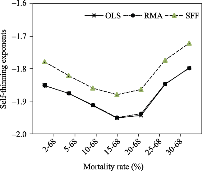
Table 2 Results of the Reineke’s slopes of the self-thinning line for the LnN versus Ln $\overline{d}$ relationships in Fujian plots
Mortality
rate (%)
Sample size Regression method R2 a Estimated slopes S.E. b 95% CI c
2-68 66 OLS 0.926 -1.851 0.063 -1.977, -1.725
RMA 0.926 -1.851 0.063 -1.946, -1.756
SFF 0.932 -1.778 0.064 -1.902, -1.653
5-68 59 OLS 0.943 -1.876 0.059 -1.995, -1.757
RMA 0.944 -1.876 0.050 -1.972, -1.780
SFF 0.957 -1.821 0.060 -1.938, -1.705
10-68 51 OLS 0.945 -1.913 0.064 -2.043, -1.784
RMA 0.945 -1.912 0.061 -2.036, -1.797
SFF 0.947 -1.860 0.062 -1.981, -1.738
15-68 43 OLS 0.928 -1.952 0.082 -2.118, -1.787
RMA 0.928 -1.951 0.079 -2.113, -1.810
SFF 0.975 -1.880 0.084 -2.045, -1.716
20-68 37 OLS 0.919 -1.944 0.093 -2.134, -1.755
RMA 0.920 -1.939 0.091 -2.134, -1.790
SFF 0.934 -1.864 0.093 -2.046, -1.682
25-68 28 OLS 0.921 -1.847 0.102 -2.055, -1.638
RMA 0.920 -1.846 0.118 -2.08, -1.634
SFF 0.935 -1.773 0.090 -1.950, -1.595
30-68 25 OLS 0.916 -1.797 0.109 -2.022, -1.572
RMA 0.913 -1.798 0.132 -2.039, -1.549
SFF 0.928 -1.720 0.097 -1.909, -1.530

a R is correlation coefficient.

b S.E. is the standard errors associated with the slope.

c 95% confidence intervals.

Fig. 1 The Reineke’s self-thinning exponents with OLS, RMA and SFF change across the seven mortality rate classes.
Multiple comparisons of group means by Duncan’s statistic detected differences between OLS and SFF (P= 0.0052), and RMA and SFF (P=0.0029), but no difference lies between OLS and RMA (P=0.9701). The S.D.s with OLS RMA and SFF are 0.0531, 0.0519 and 0.0564. We also found that no significant difference lies between -1.605Reineke’s rule and the estimated slopes (OLS (P<0.001), RMA (P<0.001) and SFF (P<0.001)), and -2WBE’s rule (OLS (P=0.0015), RMA (P=0.0013) and SFF (P=0.0002)). In addition, the 95% confidence interval (CI) was estimated with OLS, RMA and SFF. Among the seven mortality rate classes, the slope of the mortality rate class 2%-68% and its subsequent estimates do not completely contain -1.605 (-2).

3.2 Scrutiny of Yoda’s stand self-thinning law

Yoda’s self-thinning law, $\bar{w}\propto {{N}^{\beta }},$quantifies relationship between mean stem volume and numbers of stems per unit area when stands have density-dependent mortality. Similarly,the estimated self-thinning slopes with OLS, RMA and SFF also change with increasing mortality rates (Table 3). The estimated self-thinning slopes with OLS, RMA and SFF decrease from 2%-68% to 15% -68% mortality rate intervals, and then increase from 20%-68% to 30%-68% mortality rate intervals . All the highest estimated slopes with OLS (-1.480), RMA (-1.477) and SFF (-1.408) lie in the 15-68% mortality rate, and lowest slopes with OLS (-1.628), RMA (-1.613) and SFF (-1.539) lie in the 15-68% mortality rate.
Quadratic model with
$\ln {{w}_{(\text{OLS})}}=-1.671+0.072\ln N-0.075{{\ln }^{2}}N$(R2=0.8311),
$\ln {{w}_{(\text{RMA})}}=-1.609-0.073\ln N+0.073{{\ln }^{2}}N$(R2=0.7966)
and
$\ln {{w}_{(\text{SFF})}}=-1.6757-0.0745\ln N-0.079{{\ln }^{2}}N$(R2=0.8341)
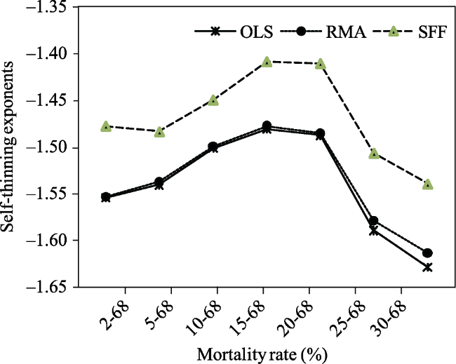
Table 3 Results of the Yoda’s slopes of the self-thinning line for the Lnw versus LnN relationships in Fujian plots
Mortality
rate (%)
Sample size Regression method R2 a Estimated slopes S.E. b 95% CI c
2-68 66 OLS 0.895 -1.554 0.063 -1.680, -1.428
RMA 0.897 -1.553 0.046 -1.637, -1.467
SFF 0.913 -1.477 0.063 -1.601, -1.353
5-68 59 OLS 0.928 -1.540 0.055 -1.649, -1.430
RMA 0.929 -1.537 0.046 -1.633, -1.459
SFF 0.951 -1.483 0.052 -1.585, -1.381
10-68 51 OLS 0.931 -1.501 0.056 -1.615, -1.388
RMA 0.932 -1.499 0.050 -1.607, -1.412
SFF 0.944 -1.449 0.054 -1.554, -1.343
15-68 43 OLS 0.904 -1.480 0.071 -1.625, -1.336
RMA 0.906 -1.477 0.061 -1.621, -1.368
SFF 0.915 -1.408 0.069 -1.543, -1.272
20-68 37 OLS 0.899 -1.487 0.080 -1.649, -1.325
RMA 0.911 -1.485 0.067 -1.628, -1.359
SFF 0.926 -1.410 0.063 -1.534, -1.286
25-68 28 OLS 0.898 -1.589 0.099 -1.793, -1.384
RMA 0.898 -1.578 0.102 -1.821, -1.434
SFF 0.915 -1.506 0.093 -1.688, -1.324
30-68 25 OLS 0.895 -1.628 0.110 -1.856, -1.400
RMA 0.893 -1.613 0.121 -1.883, -1.443
SFF 0.904 -1.539 0.102 -1.738, -1.340
These indicate that convex curve, as seen from above, are similar (Fig. 2).
Fig. 2 The Yoda’s self-thinning exponents with OLS, RMA and SFF change across the seven mortality rate classes.
Multiple comparisons of group means by Duncan’s statistic detected differences between OLS and SFF (P=0.083), RMA and SFF (P=0.079), but there was no difference between OLS and RMA (P=0.7832). The S.D.s with OLS (0.0531) RMA (0.0486) and SFF (0.0453) are similar. We also found that no difference lies in-1. 5Yoda’s law and the estimated slopes (OLS (P=0.0011), RMA (P<0.001) and SFF (P=0.0948)), but difference lies in -4/3WBE’s rule and the estimated slopes (OLS (P=0.0574), RMA (P=0.0948) and SFF (P=0.00843)). In addition, the 95% confidence interval (CI) was estimated with OLS, RMA and SFF. Among the seven mortality rate classes, the slope of the mortality rate class 2%-68% and its subsequent estimates contains -1.5, but not -4/3.

3.3 Analysis of WBE’s power rule

WBE’s power rule, $\bar{w}\propto {{\bar{d}}^{\gamma }}$, represents the relationship between mean volume and mean diameter in overcrowded pure stands. The estimated self-thinning exponents with OLS and RMA decrease between from 2%-68% to 5%-68% mortality rate intervals, and are almost constant between 5%-68% to 10%-68% mortality rate intervals, and decrease from 10%-68% to 15%-68% mortality rate intervals, and increase from 15%-68% to 25%-68% mortality rate intervals, and decrease from 25%-68% to 30%-68% mortality rate intervals. The estimated self-thinning exponents with SFF decrease from 2%-68% to 15%-68% mortality rate intervals, and then increase 15%-68% to 25%- 68% mortality rate intervals, and finally decrease from 25%-68% to 30%-68% mortality rate intervals. The oscillation with estimated self-thinning exponents indicates that the self-thinning exponents are not constant. Multiple comparisons of group means by Duncan’s statistic detected no differences between OLS and RMA (P=0.3496), but difference between OLS and SFF (P=0.0096), RMA and SFF (P=0.0094). The S.D.s with OLS (0.0293) RMA (0.0276) and SFF (0.0289) are similar. We also found that there are no differences 3Yoda’s law and the estimated slopes (OLS (P<0.001), RMA (P<0.001) and SFF (P<0.001)), but there are differences 8/3 WBE’s rule and the estimated slopes (OLS (P<0.001), RMA (P<0.001) and SFF (P<0.001)). In addition, the 95% confidence interval (CI) was estimated with OLS, RMA and SFF. Among the eight mortality rate classes, the slope of the mortality rate class 2-68% and its subsequent estimates do not contain 8/3 (3) and its entire latter estimates with OLS, RMA and SFF.
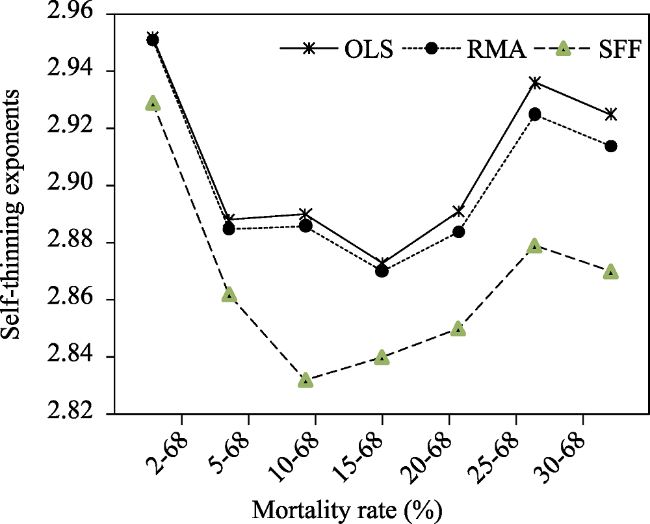
Table 4 Results of the WBE slopes of the self-thinning line for the Ln$w$ versus LnN relationships in Fujian plots
Mortality
rate (%)
Sample size Regression method R2 a Estimated slopes S.E. b 95% CI c
2-68 83 OLS 0.984 2.952 0.041 2.871, 3.034
RMA 0.985 2.951 0.032 2.891, 3.022
SFF 0.991 2.929 0.041 2.849, 3.008
5-68 59 OLS 0.982 2.888 0.051 2.785, 2.99
RMA 0.982 2.885 0.035 2.827, 2.963
SFF 0.987 2.862 0.049 2.766, 2.957
10-68 51 OLS 0.978 2.873 0.061 2.749, 2.996
RMA 0.978 2.886 0.041 2.805, 2.968
SFF 0.974 2.832 0.058 2.727, 2.953
15-68 43 OLS 0.970 2.890 0.078 2.732, 3.048
RMA 0.971 2.87 0.063 2.772, 3.019
SFF 0.978 2.840 0.065 2.705, 2.958
20-68 37 OLS 0.972 2.891 0.082 2.725, 3.057
RMA 0.972 2.884 0.077 2.761, 3.054
SFF 0.983 2.850 0.081 2.705, 2.958
25-68 28 OLS 0.961 2.936 0.111 2.708, 3.163
RMA 0.962 2.925 0.109 2.708, 3.163
SFF 0.953 2.879 0.106 2.692, 3.009
30-68 25 OLS 0.963 2.925 0.117 2.682, 3.167
RMA 0.963 2.914 0.115 2.727, 3.164
SFF 0.978 2.870 0.100 2.671, 3.087

4 Discussion

During the early stage of stand development, competition among trees is not severe enough to cause mortality, and average stem volume and diameter increase with no corresponding decrease in stand density. With growth the trees become larger, the stand becomes dense and a further increase in average stem volume and diameter result in increasing tree mortality. At this time, the beginning of competitive interactions coincides more or less with canopy closure. The growth rate for an individual tree is reduced relative to its potential in the absence of severe intraspecific competition and the size differentiation among individuals in the population accelerates (Zeide, 1987). As competition-induced mortality progresses, the increased severity in competition makes the individual trees, especially those of subordinate crown classes with limited availability to light, more susceptible to direct agents of mortality (Givnish,1986; Xue et al., 1999) and self-thinning occurs at the 2% stand mortality rate (Sun et al., 2011). The self-thinning exponents ${{b}_{N\overline{D}}}$ and ${{b}_{\overline{V}\overline{D}}}$decrease, and ${{b}_{\overline{V}N}}$increases between 2%-68% and 15%-68% mortality rate intervals (Fig. 1, Fig. 2 and Fig. 3). However, as the forest canopy becomes more open as the stands grow, small gaps in the canopy, which are typically a result of the deaths of smaller, suppressed trees, are rapidly reclaimed by the stand as the crowns of residual trees expand. This leads to a gradual increase in relative growth rates of average stem volume and diameter. At this time, an increasingly large percentage of the small and suppressed trees die, and the stand is now composed mainly of the surviving larger-sized trees. The self-thinning slope changes following the accumulation of average stem volume and diameter with little mortality occurring over the next mortality rate intervals (from 15%-68% to 30%-68%). At this time, the self-thinning exponents ${{b}_{N\overline{D}}}$ and ${{b}_{\overline{V}\overline{D}}}$increase, and ${{b}_{\overline{V}N}}$decreases. However, the self-thinning exponent ${{b}_{\overline{V}N}}$decreases from 25%-68% to 30%-68%, whichprobably implies that the self-thinning exponents fluctuate with average stem volume and diameter growth, and decrease the stem numbers. The minimum growth rate of mean stem volume and diameter were found at 15% tree mortality rate. The self-thinning exponents,${{b}_{N\overline{D}}}$,${{b}_{\overline{V}\overline{D}}}$ and ${{b}_{\overline{V}N}}$ with the seven mortality rate intervals, are not constant, and change with increasing tree morality. When density-dependent morality happens, the volume and diameter growth of the surviving trees compensate and even exceed the loss of the dead stems over a long period of time. That implies that the relationship between$N$and $\overline{D},\text{ }\overline{V}$and $\overline{D},$ and $\overline{V}$and N inevitably change.
Fig. 3 The WBE’s self-thinning exponents with OLS, RMA and SFF change across the seven mortality rate classes.
Multiple comparisons of group means by Duncan’s statistic detected differences among OLS, RMA and SFF. We found that there were no differences OLS and RMA, but there were differences between OLS and SFF, RMA and SFF. The reason is that the OLS and RMA are based on the moment estimation (Osawa and Sugita, 1989), and SFF is based on the maximum likelihood estimates of the self-thinning slopes (Coelli, 1996). The RMA self-thinning slope can be computed by OLS self-thinning slope dividing into the Pearson correlation coefficient. As a result, the OLS self-thinning exponent trajectory is almost parallel with RMA’s and the estimated self-thinning exponents with SSF are different than those of OLS and RMAs.
For Reineke’s stand density rule, the estimated self-thinning exponents with the seven mortality intervals are significantly different from -1.605Reineks’s rule and -2WBE’s rule, and are not anticipated by Euclidian or fractal scaling. Gadow (1986) and Pretzsch and Biber (2005) showed that species-specific morphologic allometric differences result in individual species’ differences with self-tolerance and efficiency of space occupation. As a result, the Reineke’s self-thinning exponents show different values at different stand self-thinning trajectories. Yoda’s self-thinning exponents vary around -3/2Yoda’s law, but are significantly different from -4/3 WBE’s rule. For WBE’s rule, exponents with the different mortality rate intervals tend to neither 8/3 WBE’s rule nor 3 Yoda’s law. Li et al. (2005) implied that the different scaling (organs, stand and forest ecosystem) exponents for the relationship between mass and diameter lead to the different scaling exponents.
We think that the lack of comparison with species properties and uniformity in premises has perhaps confounded the self-thinning laws. Meanwhile, we fascinated to see constancy and unity rather than variability and diversity, which leads to us provide positive evidence in the new article for the existence of a law based on the different density-size premise. The heterogeneity with self-thinning slopes reminds us of the relationship between the number and the size, which is not found in “universally applicable” models, and we should attempt to recognize and explain the deficiencies of the law. Only after a self-thinning law for the targeted tree species is correctly determined, can we make an adaptable density management diagram to direct practical management actions.

5 Conclusions

The relationship between stand density and tree size, i.e. self-thinning slopes, can serve as an interface between process and structure, but the self-thinning slopes with Reineke’s, Yoda’s and WBE’s fluctuate with self-thinning trajectory, not some constant. The estimated self-thinning slope values with Reineke’s and WBE’s do not conform to the theoretical values, which probably because of species-specific and scale differences. Only the Yoda’s self-thinning slopes varied around from -3/2, but were significantly different from -4/3, which implies that the Yoda’s self-thinning law is the best to explain the self-thinning trajectory of the Chinese fir stands. The numerous false trials concerning the rules from Reineke, Yoda and WBE lead to a misunderstanding of individual species-specific scaling allometry. The size and structure differences of organisms may explain away the deficiencies of the law.

The authors have declared that no competing interests exist.

[1]
Bégin E, Bégin J, Bélanger L, et al.2001. Balsam fir self-thinning relationship and its constancy among different ecological regions.Canadian Journal of Forest Research, 31: 950-959.

[2]
Bi H, Wan G, Turvey N.2000. Estimating the self-thinning boundary line as a density-dependent stochastic biomass frontier.Ecology, 81(6): 1477-1483.

[3]
Bohonak A J.2002. RMA: Software for reduced major axis regression, V1.14b, San Diego University.

[4]
Castedo D F, Crecente C F, Álvarez Á P, et al.2009. Development of a stand density management diagram for radiata pine stands including assessment of stand stability. Forestry, 82(1): 1-16.

[5]
Coelli T J.1996. A guide to FRONTIER Version 4.1: A computer program for stochastic frontier production and cost function estimation. Working paper 96/07. Centre for Efficiency and Productivity Analysis, University of New England, Armidale. Australia.

[6]
Coomes D A.2006. Challenges to the generality of WBE theory.Trends in Ecology and Evolution, 21(11): 593-596.

[7]
Del R M, Montero G, Bravo F.2001. Analysis of diameter-density relationships and self-thinning in non-thinned even-aged Scots pine stands.Forest Ecology Management, 142: 79-87.

[8]
Drew T J, Flewelling J W.1977. Some recent Japanese theories of yield-density relationships and their application to Monterey pine plantations.Forest Science, 23: 518-534.

[9]
Drew T J, Flewelling J W.1979. Stand density management: An alternative approach and its application to Douglas fir plantations.Forest Science, 25: 518-532.

[10]
Enquist B J, Brown J H, West G B.1998. Allometric scaling of plant energetics and population density.Nature, 39: 163-165.

[11]
Fang J Y, Kan M, Yamakura T.1991. Relationships between population growth and population density in monocultures of Larix leptolepis. Acta Botanica Sinica, 33: 949-957.

[12]
Gadow V K.1986. Observation on self-thinning in pine plantations.South African Journal of Science, 82: 364-368.

[13]
Gorham E.1979. Shoot height, weight and standing crop in relation to density of monospecific plant stands.Nature, 279: 148-150.

[14]
Harper J L.1967. A Darwinian approach to plant ecology.Journal of Ecology, 55: 247-270.

[15]
Inoue A, Nishizono T.2004. Allometric model of the Reineke equation for Japanese cypress (Chamaecyparis obtuse) and red pine(Pinus densiflora) stands. Journal of Forest Research, 9: 319-324.

[16]
Kikuzawa K.1999. Theoretical relationships between mean plant size, size distribution and self-thinning under one-sided competition.Annals of Botany, 83: 11-18.

[17]
Kozlowski J, Konarzewski M.2004. Is West, Brown and Enquist’s model of allometric scaling mathematically correct and biologically relevant? Functional Ecology, 18: 283-289.

[18]
Kozlowski J, Konarzewski M.2005. West, Brown and Enquist’s model of allometric scaling again: The same questions remain.Functional Ecology, 19: 739-743.

[19]
Kumar M B, Long N J, Kumar P.1995. A density management diagram for teak plantations of Kerala in peninsular India.Forest Ecology and Management, 74(1-3): 125-131.

[20]
Li B L, Wu H, Zou G.2000. Self-thinning rule: A causal interpretation from ecological field theory.Ecological Modelling, 132: 167-173.

[21]
Li H, Han X, Wu J.2005. Lack of evidence of 3/4 scaling of metabolism in terrestrial plants.Journal of Integrative Plant Biology, 47(10): 1173-1183.

[22]
Liu J, Tong S.1980. Studies on the stand density control diagram for Cunninghamia Lanceolata. Scientia Silvae Sinicae, 4: 241-251.

[23]
Long N J.1985. A practical approach to density management.The Forestry Chronicle, 61: 23-27.

[24]
Lonsdale W.1990. The self-thinning rule: dead or alive?Ecology, 71: 1373-1388.

[25]
Mohler C L, Marks P L, Sprugel D G.1978. Stand structure and allometry of tree during self-thinning of pure stand. Journal of Ecology, 68: 598-614.

[26]
Morris E C.2002. Self-thinning lines differ with fertility level.Ecological Research, 17: 7-28.

[27]
Newton P E, Smith V G.1990. Reformulated self-thinning exponents as applied to black spruce.Canadian Journal of Forest Research, 20: 887-893.

[28]
Newton P E.2006. Asymptotic size-density relationships within self-thinning black spruce and jack pine stand-types: Parameter estimation and model reformulations.Forest ecology and management, 226: 49-59.

[29]
Ogawa K, Hagihara A.2003. Self-thinning and size variation in a sugi (Cryptomeria japonica D. Don) plantation. Forest Ecology and Management, 174: 413-421.

[30]
Osawa A.1995. Inverse relationship of crown fractal dimension to self- thinning exponent of tree population: A hypothesis.Canadian Journal of Forest Research, 25: 1608-1617.

[31]
Pretzsch H, Biber P.2005. A re-evaluation of Reineke’s rule and stand density index.Forest Science, 51(4): 304-320.

[32]
Pretzsch H.2002. A unified law of spatial allometry for woody and herbaceous plants.Plant Biology, 4: 159-166.

[33]
Pretzsch H.2006. Species-specific allometric scaling under self-thinning: Evidence from long-term plots in forest stands.Oecologia, 146: 572-583.

[34]
Reineke L H.1933. Perfecting a stand density index for even-aged forests.Journal of Agricultural Research, 46: 627-638.

[35]
Roderick M L, Barnes B.2004. Self-thinning of plant population from a dynamic viewpoint.Functional Ecology, 18: 197-203.

[36]
Smith N J, Hann D W.1986. A growth model based on the self-thinning rule.Canadian Journal of Forest Research, 16: 330-334.

[37]
Sokal R R, Rohlf F J.1981. Biometry, 2nd edn. Freeman, San Francisco.

[38]
Solomon D S, Zhang L.2002. Maximum size-density relationships for mixed softwoods in the northeastern USA.Forest Ecology and Management, 155: 163-170.

[39]
Sun H, Zhang J, Duan A, et al.2011. Estimation of the self-thinning boundary line within even-aged Chinese fir (unninghamia lanceolata(Lamb.) Hook.) stands: Onset of self-thinning. CForest Ecology and Management, 261: 1010-1015.

[40]
Weller D E.1987. Self-thinning exponent correlated with allometric measures of plant geometry.Ecology, 68: 813-821.

[41]
West G B, Brown J H, Enquist B J.1997. A general model for the origin of allometric scaling laws in biology.Science, 276: 122-126.

[42]
West G B, Brown J H, Enquist B J.1999. A general model for the structure and allometry of plant vascular systems.Nature, 400: 664-667.

[43]
Westoby M.1977. Self-thinning driven by leaf area not by weight.Nature, 265: 330-331.

[44]
Westoby M.1984. The self-thinning rule.Advances in Ecological Research, 14:167-225.

[45]
White J, Harper J L.1970. Correlated changes in plant size and number in plant populations.Journal of Ecology, 58: 467-485.

[46]
Whitfield J.2001. All creatures great and small.Nature, 413: 342-344.

[47]
Yang Y, Titus S J.2002. Maximum size-density relationship for constraining individual tree mortality functions.Forest Ecology and Management, 168: 259-273.

[48]
Yoda K, Kira T, Ogawa H, et al.1963. Self-thinning in overcrowded pure stand under cultivated and natural conditions.Journal of Biology of Osaka City University, 14: 107-129.

[49]
Zeide B.1987. Analysis of the 3/2 power law of self-thinning.Forest Science, 33: 517-537.

[50]
Zeide B.1991. Self-thinning and stand density.Forest Science, 37: 517-523.

Outlines

/