Forest Ecosystem

Remote Sensing Indices to Measure the Seasonal Dynamics of Photosynthesis in a Southern China Subtropical Evergreen Forest

  • SUN Leigang 1, 2, 3 ,
  • WANG Shaoqiang , 1, 2, 4, * ,
  • Robert A. MICKLER 5 ,
  • CHEN Jinghua 1, 2 ,
  • YU Quanzhou 6 ,
  • QIAN Zhaohui 1, 2 ,
  • ZHOU Guoyi 7 ,
  • MENG Ze 7
Expand
  • 1. Key Laboratory of Ecosystem Network Observation and Modeling, Institute of Geographic Sciences and Natural Resources Research, Chinese Academy of Sciences, Beijing 100101, China
  • 2. University of Chinese Academy of Sciences, Beijing 100049, China
  • 3. Hebei Engineering Research Center for Geographic Information Application, Institute of Geographical Sciences, Hebei Academy of Sciences, Shijiazhuang 050011, China
  • 4. School of Geography and Information Engineering, China University of Geosciences, Wuhan 430074, China
  • 5. Department of Forestry and Environmental Resources, North Carolina State University, Raleigh, North Carolina, USA
  • 6. School of Environment and Planning, Liaocheng University, Liaocheng, Shandong 252059, China
  • 7. South China Botanical Garden, Chinese Academy of Sciences, Guangzhou 510650, China
*Corresponding author: WANG Shaoqiang, E-mail:

Received date: 2018-10-11

  Accepted date: 2018-11-12

  Online published: 2019-03-30

Supported by

National Key Research and Development Program of China (2017YFC0503803)

National Natural Science Foundation of China (41571192)

Natural Science Foundation of Hebei, China (D2016302002)

Science and Technology Planning Project of Hebei, China (17390313D).

Copyright

All rights reserved

Abstract

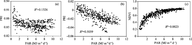
The accurate measurement of the dynamics of photosynthesis in China’s subtropical evergreen forest ecosystems is an important contribution to carbon (C) sink estimates in global terrestrial ecosystems and their responses to climate change. Eddy covariance has historically been the only direct method to assess C flux of whole ecosystems with high temporal resolution, but it suffers from limited spatial resolution. During the last decade, continuous global monitoring of plant primary productivity from spectroradiometer sensors on flux towers and satellites has extended the temporal and spatial coverage of C flux observations. In this study, we evaluated the performance of two physiological remote sensing indices, fluorescence reflectance index (FRI) and photochemical reflectance index (PRI), to measure the seasonal variations of photosynthesis in a subtropical evergreen forest ecosystem using continuous canopy spectral and flux measurements in the Dinghushan Nature Reserve in southern China. The more commonly used NDVI has been shown to be saturated and mainly affected by illumination (R2=0.88, p < 0.001), but FRI and PRI could better track the seasonal dynamics of plant photosynthetic functioning by comparison and are less affected by illumination (R2=0.13 and R2=0.51, respectively) at the seasonal scale. FRI correlated better with daily gross primary production (GPP) in the morning hours than in the afternoon hours, in contrast to PRI which correlated better with light-use efficiency (LUE) in the afternoon hours. Both FRI and PRI could show greater correlations with GPP and LUE respectively in the senescence season than in the recovery-growth season. When incident PAR was taken into account, the relationship between GPP and FRI was improved and the correlation coefficient increased from 0.22 to 0.69 (p < 0.001). The strength of the correlation increased significantly in the senescence season (R 2=0.79, p < 0.001). Our results demonstrate the application of FRI and PRI as physiological indices for the accurate measurement of the seasonal dynamics of plant community photosynthesis in a subtropical evergreen forest, and suggest these indices may be applied to carbon cycle models to improve the estimation of regional carbon budgets.

Cite this article

SUN Leigang , WANG Shaoqiang , Robert A. MICKLER , CHEN Jinghua , YU Quanzhou , QIAN Zhaohui , ZHOU Guoyi , MENG Ze . Remote Sensing Indices to Measure the Seasonal Dynamics of Photosynthesis in a Southern China Subtropical Evergreen Forest[J]. Journal of Resources and Ecology, 2019 , 10(2) : 112 -126 . DOI: 10.5814/j.issn.1674-764X.2019.02.002

1 Introduction

Plant photosynthesis supports most life on Earth and drives the largest flux of carbon dioxide (CO2) between the terrestrial biosphere and the atmosphere. The dynamic variability of seasonal photosynthetic activity affects not only the global atmospheric-biospheric chemistry and climate, but also terrestrial sources and sinks (Peñuelas et al., 2009; Richardson et al., 2013). Increasing attention has been given to the accurate measurements and estimates of GPP to track photosynthetic phenology and monitor photosynthetic performance, which is crucial to quantitatively assess ecosystem functioning, carbon budgets, food production, and the impacts from human activities on climate change (Grace et al., 2007; Zhang et al., 2014; Duveiller et al., 2016). GPP also plays a key role in the projections of future carbon cycles and climate change (Schimel et al., 2015). There is, however, a lack of monitoring indices directly related to GPP or plant photosynthesis processes. Although spatio-temporal dynamic monitoring of GPP and net primary productivity (NPP) can be achieved by remote sensing technology, the estimation of GPP has been mainly based on the sensitivity of structural indices such as NDVI and enhanced vegetation indices (EVI) to the seasonal phenological changes within time series (Running et al., 2004; Huete et al., 2006). These structural indices vary with the vegetation canopy structure, but are closely related to vegetation parameters (e.g. chlorophyll content, biomass, and canopy structure and coverage) (Meroni et al., 2009; Guanter et al., 2014; Joiner et al., 2014). These indices are less sensitive to plant physiological changes (Damm et al., 2010), especially for evergreen vegetation, where the plant physiology changes while the canopy leaf area index (LAI) changes slightly. This may introduce important errors in the estimates of carbon exchange and result in increased uncertainty in the estimates of GPP (Parazoo et al., 2014).
In natural environments, plants do not absorb all incoming sunlight. Reduction in photosynthetic efficiency is a result of reflection, and the respiration requirements of photosynthesis. Since not all photosynthetically active radiation energy is converted into biomass, the result is an overall photosynthetic efficiency of 3% to 6% of total solar radiation. To balance the absorption and utilization of light energy for healthy metabolic growth, and protect the photosynthetic apparatus from photodamage, excess light energy can be dissipated as heat by non-photochemical quenching (NPQ), or re-emitted as chlorophyll fluorescence (Müller et al., 2001; Van der Tol et al., 2009). Light absorption results in singlet-state excitation of chlorophyll a molecules. An absorbed photon can follow three alternative pathways: chlorophyll fluorescence emission, photosynthesis or heat dissipation, all leading to the deexcitation of chlorophyll a molecules (Genty et al., 1989). Because these three pathways compete for the same excitation energy, chlorophyll fluorescence emission and NPQ carry information on photosynthesis efficiency. With the development of remote sensing sensors, some physiological indices, such as PRI and Chlorophyll Fluorescence Index, related to NPQ and chlorophyll fluorescence emission respectively, can be extracted by hyperspectral remote sensing. This may facilitate an assessment of the photosynthetic status of vegetation to monitor photosynthesis dynamics.
NPQ is a light protective mechanism that dissipates excess energy as heat to prevent over-excitation of Photosystem II (PSII) (Ruban et al., 2017) by the xanthophyll cycle (Müller et al., 2001; Goss et al., 2015). Once PSII is activated, the changes in the quantum yield of photochemistry will be controlled by the dynamics of NPQ (Porcar-Castell et al., 2014), which in turn directly affects LUE. Previous studies showed that this reversible xanthophyll cycle (i.e., xanthophyll de-epoxidation) will result in the rapid decrease of spectral reflectance at 531 nm (Gamon et al., 1990; Gamon et al., 1992). A normalized difference reflectance expressed as the PRI, was constructed with this spectral reference band at 531 nm and another spectral reference band at 570 nm unaffected by the xanthophyll de-epoxidation reaction (Gamon et al., 1992; Gamon et al., 1997). The linear correlation between PRI and NPQ has been found under various conditions (Evain et al., 2004; Sarlikioti et al., 2010; Chou et al., 2017; Sukhova et al., 2018). PRI could explain 77% of the variation in NPQ for herbaceous leaves at the seasonal scale (Garbulsky et al., 2011). Good correlations were also reported during different short-term light phases (Evain et al., 2004; Atherton et al., 2016). In addition, LUE is used to partition the absorbed light energy between photochemical and non-photochemical pathways (Demmig-Adams et al., 2006; Ensminger et al., 2006) and plays a key role in the accurate estimation of GPP (Wei et al., 2017; Nuarsa et al., 2018). Many studies have reported that PRI could be effective for tracking the LUE across various plant functional types, including crops, grass, deciduous forests, and boreal evergreen forests, and under different conditions at the leaf, canopy and the ecosystem levels (Garbulsky et al., 2011; Soudani et al., 2014; Stagakis et al., 2014; Zhang et al., 2015). However, the correlation between PRI and LUE can vary significantly due to variations in the viewing directions and illumination conditions, and also be affected by the physiological and biochemical properties of leaves (e.g., the chlorophyll content) (Garbulsky et al., 2011; Merlier et al., 2015; Takala et al., 2016). In tropical and subtropical evergreen forests, there is limited research on the relationship between PRI and LUE. The spatio-temporal variation characteristics of LUE are still uncertain (Nakaji et al., 2014).
Chlorophyll fluorescence has been used in plant photosynthesis research at the leaf, canopy, and landscape levels for decades (Porcar-Castell et al., 2014). Pulse amplitude- modulated (PAM) fluorimeter is among the most widely used techniques for chlorophyll fluorescence measurements to determine the photosynthetic quantum yields of absorbed photons (Bilger et al., 1995; Baker et al., 2008). Yet, PAM fluorescence is restricted to the leaf level for tracking variation in the light reactions of photosynthesis (Murchie et al., 2013) and clarifies the linkage between chlorophyll fluorescence and photosynthetic CO2 assimilation. Remote sensing techniques utilizing high spectral resolution spectrometers to passively detect solar-induced chlorophyll fluorescence (SIF) have facilitated the study of the acclimation of photosynthesis at the canopy and landscape levels (Damm et al., 2010). The global terrestrial chlorophyll fluorescence was first observed from the Greenhouse Gases Observing Satellite (GOSAT) in 2011 and used to estimate GPP at the landscape level (Frankenberg et al., 2011; Joiner et al., 2011). Subsequent satellite sensor outputs of SIF have been achieved with different space-borne instruments (Joiner et al., 2013; Joiner et al., 2016), many of which were not originally designed for measuring SIF. Many studies have also begun to spring up around the relationship between GPP derived using state-of-the-art methods and SIF observed from GOSAT, the Global Ozone Monitoring Experiment-2 (GOME-2) , and the Orbiting Carbon Observatory-2 (OCO-2) (Lee et al., 2013; Guanter et al., 2014; Sun et al., 2017), and they have indicated that SIF is highly correlated with GPP, although it has been shown that the SIF-GPP relationship is biome specific (Guanter et al., 2012; Damm, et al., 2015; Wood et al., 2017; Xing et al., 2018). However, higher spectral resolution and better signal-to-noise ratio (SNR) are needed for the data retrieval of satellite SIF (Damm et al., 2011; Julitta et al., 2016). The available sensors have low spatial and temporal resolution, and may adopt a discontinuous spatial sampling mode to improve spatial resolution. This impedes both ground-based validation as well as regional studies (Duveiller et al., 2016). The FLuorescence EXplorer (FLEX) mission is specifically designed for measuring SIF and will be launched in 2022 (Cogliati et al., 2015). Most of the previous SIF studies that included field studies have been conducted over croplands (Guanter et al., 2014; Liu et al., 2017), grasslands (Damm et al., 2015), shrublands (Rascher et al., 2009; Zarco-Tejada et al., 2012) and deciduous forests (Yang et al., 2015). While there have been studies on boreal evergreen forests (Walther et al., 2016), little attention has been given to subtropical evergreen forests.
China has preserved the best example of a south subtropical evergreen forest ecosystem in the world, which is one of the most distinctive and research-worthy regions at its latitude (Zhou et al., 2003). Located near the Tropic of Cancer, it includes a famous desert zone. The subtropical forest ecosystem has a high productive potential, plays an important role in regulating regional ecological balance and is also in a region sensitive to climate change (Zhou et al., 2003). Based on flux observations and model simulations, it has been discovered that the Subtropical evergreen forest is an important component of carbon sinks in the East Asian monsoon region, accounting for 8% of the global forest net ecosystem productivity (NEP) (Yu et al., 2014). However, there is still no effective technical means to real-time monitor its temporal and spatial dynamic characteristics, which continues to impede further in-depth research on the processes and mechanisms of photosynthesis response to climate change. This is especially true in the context of frequent extreme climate events, in response to temperature and water stress. Research on the photosynthetic function of the subtropical evergreen forest plays an important role in the study of global forest ecosystem productivity.
In this study, we will determine the validity of using remote sensing indices to measure the seasonal variations of photosynthesis in a subtropical evergreen forest ecosystem based on continuous canopy spectral and flux measurements. The goals of our study are to: 1) characterize the seasonal photosynthetic dynamics of evergreen forest in the subtropical region; 2) track seasonal photosynthetic dynamics variability using physiological remote sensing indices of fluorescence emission; and 3) evaluate the feasibility and performance of physiological indices in the estimation of GPP in a subtropical evergreen forest ecosystem. The results of this study will help to enhance the understanding of the dynamic characteristics of photosynthetic function in the subtropical evergreen forest ecosystem and reduce the uncertainty in carbon budget estimation.

2 Materials and methods

2.1 Study site

The study site is a part of the Chinese Ecosystem Research Network (CERN) and the China FLUX network. It is the most typical and complete south subtropical evergreen coniferous and broadleaf forest ecosystem, is considered to be one of the most distinctive and research-worthy areas in the latitudinal zone, and is dominated by 100 year old stands of Schima superba, Castanopsis chinensis, and Pinus massoniana, with a mean canopy height of 17 m and 4 layers of canopy including shrubs and herbs (Wang et al., 2007; Ouyang et al., 2014). This region has a typical south subtropical monsoon humid climate, with an annual mean air temperature of 21 ℃ and annual mean precipitation of 1956 mm (Wang et al., 2007).

2.2 Flux and meteorological data computation

The flux observation tower is installed in the core area of Dinghushan Nature Reserve (23°10°24''N, 112°32°10''E, elevation 240 m), on which one Open Path Eddy Covariance (OPEC) was mounted at 27 m. The OPEC instrumentation consisted of a Campbell Scientific CSAT3 sonic anemometer (Campbell Scientific Ltd., USA) and a Li-COR Li7500 open-path gas analyzer (Li-COR, Lincoln, NE, USA), logged at a frequency of 10 Hz and scaled to 30 min mean fluxes. Synchronous meteorological observation data, including air temperature (Ta), photosynthetically active radiation (PAR), soil moisture (SM), soil temperature (ST) and vapor pressure (VP), were also averaged to 30 min mean fluxes.
GPP was calculated using the measured Net Ecosystem CO2 Exchange (NEE) and daytime ecosystem respiration (Re) (Reichstein et al., 2005).
GPP = -NEE + Re (1)
where Re was estimated with an empirical equation fitted using nighttime NEE and soil temperature.
The LUE model was originally developed as a conceptual model. The existing models have various operational definitions based on different measurement approaches for its component terms (Monteith et al., 1972; Nichol et al., 2000; Gilmanov et al., 2014). In this study, based on acquired Photosynthetic Photon Flux Density (PPFD), the Canopy LUE was calculated using the procedures described by Nichol et al. (2000) and Barton et al. (2001):
LUE = GPP/PARinc (2)
where GPP was derived from the CO2 flux observations made using the eddy covariance technique, and PARinc was the daily averaged incident PAR (Suyker et al., 2004; Gilmanov et al., 2014).

2.3 Spectral measurements and processing

An automated multi-angular spectral observation system was installed on the flux tower on April 2014 to acquire vegetation canopy spectral data. This observation system (AMSPECⅡ) which was developed by Hilker et al. (2010), uses a dual channel spectrometer, Unispec-DC (PP Systems, Amesbury, MA, USA), and includes upwelling and downwelling channels which share the same visible and near- infrared range (305-1135 nm) with a full width at half maximum (FWHM) of 3 nm. The upwelling and downwelling channels measured simultaneously incoming solar irradiance and canopy-reflected radiance, respectively. The observation angle ranged from 42° to 62° or 37° to 57° in the vertical direction, and 10° to 160° or 190° to 340° in the horizontal direction, with an interval of 10°. This system changes the observation angle every 5 seconds and completes one observation cycle every 15 minutes.
Chlorophyll fluorescence is emitted in two broad bands with peaks in the red and in the far-red regions, approximately centered at 685 nm (F685) and 740 nm (F740) (Lichtenthaler et al., 1988; Franck et al., 2002). Since the F685 is located in the region of the greater reabsorption spectrum, the Fluorescence Reflectance Index (FRI) was calculated using the F740 peak and the band at 800 nm (F800). F800 was not affected by chlorophyll fluorescence emission. The FRI (proposed by Dobrowski et al., 2005) was calculated as:
FRI = R740/R800 (3)
Where R indicates reflectance, and the subscript is the waveband in nm. FRI represented the daily mean value from 8:30 a.m. to 17:00 p.m. We also calculated FRI_am (from 8:30 a.m. to 9:30 a.m.), FRI_mid (from 11:30 a.m. to 13:30 p.m.), and ΔFRI (the difference between FRI_mid and FRI_am) using Formula 3.
Previous studies have shown that GPP can be estimated through direct correlation with chlorophyll-related indices (Gitelson et al., 2008), without using independent estimates of the FAPAR (fraction of photosynthetically active radiation absorbed by vegetation) and the ε terms in the Monteith’s model (Monteith et al., 1992; Monteith et al., 1997). However, because the illumination effect was not taken into account, these models could not accurately simulate the short-term variation of high frequency GPP. Recent studies that modelled GPP as the product of VIs and incident PAR, had improved performance (Wu et al., 2009; Peng et al., 2011; Rossini et al., 2012; Wang et al., 2017). Fyield, Fam-yield and Fmid-yield were calculated by introducing incident PAR:
Fyield = PAR/FRI (4)
PRI is commonly calculated using two green bands at 531 nm and 570 nm (Gamon et al., 1992; Gamon et al., 1997) as:
PRI = (R531-R570) / (R531+R570) (5)
Where R is reflectance, and the subscript indicates the waveband in nm. PRI represented the daily mean value from 8:30 a.m. to 17:00 p.m. We also calculated PRI_am (from 8:30 a.m. to 9:30 a.m.), PRI_mid (from 11:30 a.m. to 13:30 p.m.), and ΔPRI (the difference between PRI_mid and PRI_am) using Formula 5.
The widely used NDVI is calculated using two green bands at 670 nm and 800 nm (Rouse et al., 1974; Tucker, 1979) as:
NDVI = (R800-R670)/(R800+R670) (6)
where R is reflectance, and the subscript indicates the waveband in nm. NDVI also represented the daily mean value from 8:30 a.m. to 17:00 p.m.

3 Results

3.1 Seasonal variation of GPP, LUE, NDVI, physiological indices and climatic factors

Fig. 1 illustrates the seasonal variations of GPP, LUE, FRI, PRI, NDVI, and the climatic factors. The data gaps from DOY 359 in 2014 to DOY 10 in 2015 and from DOY 181 to 195 in 2015 were the results of instrumental failure. The seasonal changes of Ta, SM, VPD, LUE, FRI and PRI are shown as daily average values from 8:30 a.m. to 17:00 p.m. (local solar time), along with daily GPP and PAR values. Ta, SM, VPD, PAR and GPP exhibited similar seasonal patterns across years (Fig. 1a, Fig. 1b), while LUE and PRI showed the opposite trends (Fig. 1b, Fig. 1c). SM and Ta varied synchronously, indicating the subtropical monsoon climate characteristic for the study area. It should be noted that FRI and GPP varied asynchronously across the entire observation period (from 1 June 2014 to 30 September 2015), and showed the opposite seasonal patterns (Fig. 1b, Fig. 1c). Some short-term negative relationships between FRI and GPP were observed from early October 2014 to early March 2015, when the Ta and SM were at their lowest points for the whole year.
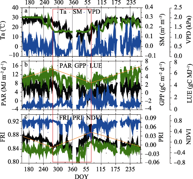
Fig. 1 Seasonal variation of climatic factors, GPP, LUE and remote sensing indices
Note: The data observation period was from 2014 (DOY 152, 1 June) to 2015 (DOY 273, 30 September). Daily average Ta, VPD, SM, LUE, FRI, PRI and NDVI were calculated using data observed from 8:30 a.m. to 17:00 p.m. each day (local solar time). PAR and GPP are the sums of values between 8:30 a.m. to 17:00 p.m. The solid lines indicate moving averages of 30 days. The red rectangle indicates the senescence season from early October 2014 (DOY 274) to early March 2015 (DOY 70).
Although the vegetation seasonal dynamics for evergreen forest were not significant, Fig. 1b showed a clear seasonal cycle of photosynthesis (GPP) with a single-peak in early October. During the study period (1 June 2014 to 30 September 2015), the GPP showed an increasing trend from 1 June to 30 September 2014, followed by an obviously decreasing period, and reaching the lowest level in February 2015. Gradual increases in GPP were observed with the gradual rising of Ta in the early Spring, indicating the restoration of photosynthetic function. The period from early October 2014 (DOY 274) to early March 2015 (DOY 70) was defined as the senescence season of photosynthetic function (Fig. 1), with photosynthetic activity of leaves decreasing gradually, and the remainder of the study period as the recovery-growth season.
GPP exhibited an overall seasonal variation similar to PAR and Ta, in contrast to VPD and SM. As presented in Fig. 2, PAR could explain 59.63% of GPP variance (Fig. 2a), followed by Ta (R2=0.2862, see Fig. 2b). The relationships between GPP and other climatic factors (i.e., SM) were weaker. Many previous studies have reported the positive relationship between GPP and PAR for different ecosystem types, and for the evergreen forest ecosystem, a slightly alternative FAPAR in the light-use efficiency (LUE) model proposed by Monteith (1972, 1977) strengthened the seasonal variations. The highest GPP appeared in early October and with the gradual lowering of PAR, GPP reached the lowest level in February 2015. However, during the recovery-growth season from June to September as shown in Fig. 1b, both PAR and Ta changed only slightly, while GPP increased significantly and continuously. FRI showed the opposite trend (Fig. 1c, orange line), which indicates that optimum Ta and PAR for the subtropical evergreen forest in this study appeared in this period. Under the definite and suitable light condition, with increasing photosynthetic capacity, less energy absorbed by Chl was dissipated as fluorescence or through non-photochemical quenching (NPQ), resulting in the decreasing FRI and PRI (Fig. 1c).
Fig. 2 Relationships of daily climatic factors (PAR, Ta and VPD) with GPP (a-c) and LUE (d-f) from 1 June 2014 to 30 September 2015
Unlike GPP, the seasonal cycles of LUE and PRI had no clear trends, but showed similar seasonal patterns. In addition, Fig. 1 shows that LUE and PRI varied inversely with PAR and VPD. LUE increased significantly with decreases of PAR and VPD. When the lowest level of PAR was detected in February 2015, LUE and PRI synchronously reached their highest levels, and PAR could explain 67.65% of LUE variance (Fig. 2d), while VPD could explain 33.06% (Fig. 2e). Moreover, the variability of LUE and PRI was smaller at the recovery-growth season of photosynthetic function from June 2014 to September 2014 than at the senescence season (Fig. 1d).
As shown in Fig. 1c, the saturation of NDVI, as the frequently-used reflectance-based VI, was observed distinctly at the recovery-growth season of photosynthetic function, which may have resulted from the small changes in vegetation coverage for evergreen forest. Many studies have also proven that conventional vegetation indices (e.g., NDVI), which are related to canopy structure, pigment concentrations and illumination, fail to detect these seasonal photosynthetic dynamics (Gamon et al., 1995; Garbulsky et al., 2010). As presented in Fig. 3, PAR could explain 88.23% of NDVI variance (Fig. 3c). By contrast, PAR could only explain 50.59% of PRI variance (Fig. 3b), and 13.26% for FRI (Fig. 3a). Due to the saturation effect, NDVI could not track the seasonal variation of GPP for evergreen forest very well (Fig. 1c), which further indicated that illumination condition was the main factor affecting the seasonal change of NDVI (Fig. 3c), and conventional reflectance-based VI may be insensitive to plant photosynthetic physiological changes.This study focused on the responses of FRI and PRI, the typical physiological reflectance-based VIs, to the dynamic changes of plant photosynthesis for the subtropical evergreen forest ecosystem.
Fig. 3 Relationships of PAR with FRI (a), PRI (b), and NDVI (c) from 1 June 2014 to 30 September 2015

3.2 FRI tracks photosynthesis dynamics

According to Fig. 1b, FRI varied inversely with GPP, especially when the fluctuation was the greatest. Calculating the negative values of FRI, FRI_am and FRI_mid could vividly display their relationships with GPP. Fig. 4 shows the seasonal patterns of GPP compared with different forms of FRI: -FRI, -FRI_am, -FRI_mid and ΔFRI. Clear seasonal dynamics were observed for GPP (Fig. 4), which increased at the recovery-growth season and reached the highest productivity at the end of September, before declining rapidly to notably lower values during the photosynthetic senescent stage with decreasing PAR and Ta (Fig. 1a,b). These different forms of FRI may track the seasonal dynamics of photosynthesis to varying degrees. -FRI, -FRI_am and -FRI_mid showed similar seasonal trajectories. The seasonal pattern (June 2014 to September 2015) of -FRI_am agreed better with that of daily GPP (R2=0.3248, p<0.001; Fig. 5b) than -FRI_mid (R2=0.1332, p<0.001; Fig. 5c) or -FRI (R2=0.2243, p<0.001; Fig. 5a). This may indicate that FRI in the morning (averaged from 8:30 a.m. to 9:30 a.m.) could track seasonal growing and senescence patterns. Since the ΔFRI were derived from FRI_am and FRI_mid, which reduced the influence of diurnal variation and represented the relative intensity of fluorescence-emission, a contribution to the canopy level apparent reflectance, positive relationships between daily GPP and ΔFRI on the seasonal scale are presented in Fig. 5 (R2=0.15, p<0.0001; Fig. 5d). In general, all forms of the FRI variables had seasonal trends similar to GPP.
Fig. 4 Seasonal variation of GPP and various FRI
Note: Daily average FRI were calculated using data observed from 8:30 a.m. to 17:00 p.m. each day (local solar time). GPP are the sum values between 8:30 a.m. to 17:00 p.m. The average FRI_am were calculated using data observed from 8:30 a.m. to 9:30 a.m. The average FRI_mid were calculated using data observed from 11:30 a.m. to 13:30 p.m. △FRI were the differences between FRI_mid and FRI_am. -FRI, -FRI_am and -FRI_mid indicate the negative values of FRI, FRI_am and FRI_mid, respectively. The solid lines indicate moving averages of 30 days.
Fig. 5 Relationships of daily GPP with FRI (a), FRI_am (b), FRI_mid (c), and ΔFRI (d)
By taking into account the incident PAR, the relationships of daily GPP with FRI, FRI_am and FRI_mid were further strengthened (Fig. 6). Although less than 3% of the absorbed photons were reemitted as fluorescence, GPP showed a significantly nonlinear correlation with Fyield (R2=0.6879, p<0.001; Fig. 6a), Fam-yield (R2=0.5533, p<0.001; Fig. 6b) and FRI_mid_yield (R2=0.6102, p<0.001; Fig. 6c). Moreover, as shown in Fig. 7, Fyield, Fam-yield, and Fmid-yield may track the seasonal dynamics of photosynthesis better than the different forms of FRI (Fig. 4). During the study period, which included different seasons, the values of Fmid-yield were greater than Fam-yield (Fig.7), which indicates that the fluorescence emitted by vegetation at noon was stronger than in the morning. This was also observed in Fig. 4 and is consistent with the known mechanism of fluorescence emission.
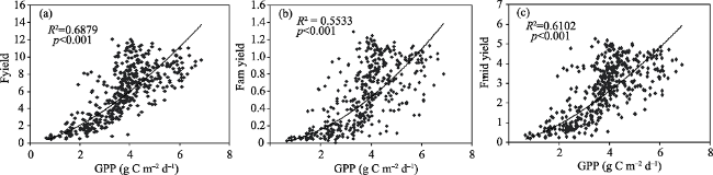
Fig. 6 Relationships of daily GPP (gC m-2 d-1) with Fyield (a), Fam-yield (b) and Fmid-yield (c). Fyield were calculated by dividing FRI by PAR from 8:30 a.m. to 17:00 p.m. Fam-yield were calculated by dividing FRI_am by PAR from 8:30 a.m. to 9:30 p.m. Fmid-yield were calculated by dividing FRI_mid by PAR from 11:30 a.m. to 13:30 p.m.
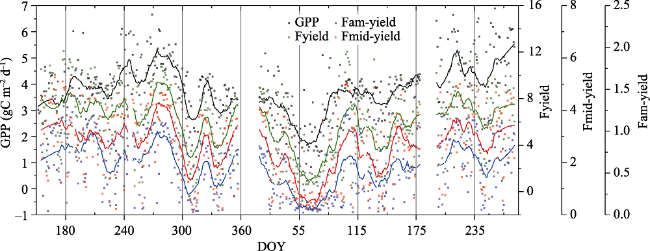
Fig. 7 Seasonal variations of GPP (gC m-2 d-1, black dots and lines), Fyield (red dots and lines), Fam-yield (blue dots and lines) and FRI_mid (green dots and lines) from 2014 (DOY 152, 1 June) to 2015 (DOY 273, 30 September). The solid lines indicate moving averages of 30 days.
The statistics of modeling GPP using FRI are summarized in Table 1. By further distinguishing between the recovery-growth season and the senescence season of photosynthetic function, both FRI and Fyield track seasonal variations of GPP in the senescence season better than in the recovery-growth season (Table 1). For example, in the senescence season, FRI had significant correlations with GPP (R2=0.5373, p<0.001), which were greater than during the recovery-growth season (R2=0.1573, p<0.001). The correlation between Fyield and GPP was the highest (R2=0.7924, p<0.001) in the senescence season. Fmid-yield and Fam-mid also showed greater correlations (R2=0.7353 for Fmid-yield, R2=0.6522 for Fam-mid) with GPP in the senescence season than in the recovery-growth season (R2=0.5163 for Fmid-yield, R2=0.4773 for Fam-mid), which may be because in the senescence season, GPP shows obvious seasonal changes while in the recovery-growth season, GPP keeps growing steadily in subtropical evergreen forest ecosystems. This may be due to the gradual decline of the functional organs of the plant in the senescence season, which is more sensitive to environmental factors. The greater fluctuation in the senescence season may make the correlation between FRI and GPP more significant.
Table 1 Coefficients of correlation (R2) between GPP and various FRI and Fyield during different seasons
Index FRI FRI_am FRI_mid Fyield Fam-yield Fmid-yield
All seasons 0.2243 0.3248 0.1332 0.6879 0.5533 0.6102
Recovery-growth season 0.1573 0.3021 0.0936 0.5974 0.4773 0.5163
Senescence season 0.5373 0.4876 0.4434 0.7924 0.6522 0.7353

Note: All correlations were significant (p<0.001, Pearsons correlation test).

3.3 PRI tracks light-use-efficiency (LUE) dynamics

As shown in Fig. 8, daily average PRI and PRI in the morning (PRI_am) and at noon (PRI_mid) track LUE dynamics. The PRI_mid were greater than PRI_am, which is consistent with many previous studies (Garbulsky et al., 2011). Compared to the relationships between GPP and FRI, LUE and PRI showed a significant positive correlation (R2=0.5514, p<0.001; Fig. 9a). However, PRI at the noon (PRI_mid) exhibited the best correlation with LUE (R2=0.5639, p< 0.001; Fig. 9c), and FRI in the morning (FRI_am) showed the strongest correlation with GPP (Fig. 4). ΔPRI showed a lower correlation with LUE (R2=0.0735, Fig. 9d). Similar to FRI and Fyield (Table 1), PRI also track the LUE dynamics better in the senescence season than in the recovery-growth season (see Table 2).
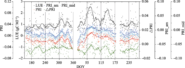
Fig. 8 Seasonal variation of LUE (gC MJ-1, black dots and lines), PRI (red dots and lines), PRI_am (blue dots and lines), PRI_mid (light blue dots and lines) and ΔPRI (green dots and lines) from 2014 (DOY 152, 1 June) to 2015 (DOY 273, 30 September). The solid lines indicate moving averages of 30 days. Daily average LUE and PRI were calculated using data observed from 8:30 a.m. to 17:00 p.m. each day. The average PRI_am were calculated using data observed from 8:30 a.m. to 9:30 a.m. The average PRI_mid were calculated using data observed from 11:30 a.m. to 13:30 p.m. ΔFRI were the differences between FRI_mid and FRI_am. ΔPRI were the differences between PRI_mid and PRI_am.
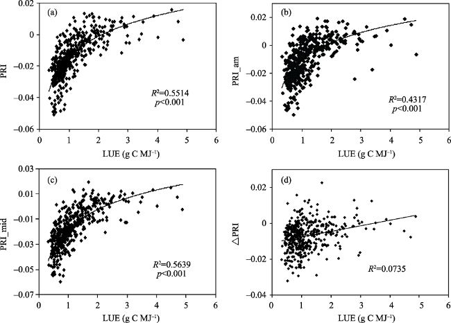
Fig. 9 Relationships of daily average LUE with PRI (a), PRI_am (b), PRI_mid (c) and ΔPRI (d)
Table 2 Coefficients of correlation (R2) between LUE and PRI, PRI_am, and PRI_mid. during different seasons.
Index PRI PRI_am PRI_mid
All seasons 0.5514 0.4317 0.5639
Recovery-growth season 0.5370 0.3883 0.5181
Senescence season 0.8034 0.7001 0.7995

Note: All correlations were significant (p<0.001, Pearsons correlation test).

In addition, similar to the correlations between FRI, Fyield and GPP (Table 1), PRI also tracks the LUE dynamics better in the senescence season than in the recovery-growth season (Table 2). Specifically, PRI could explain 80.34% of LUE variance in the senescence season, and just 53.7% in the recovery-growth season.

4 Discussion

In this study we evaluated the seasonal variations of GPP, LUE, climatic factors, narrow-band physiological indices (FRI and PRI), NDVI, and their correlations based on the data obtained from long-term observations for the south subtropical evergreen forest ecosystem. The study period, from 1 June 2014 to 30 September 2015, covered four seasons: spring, summer, autumn and winter.
One of the goals of this study is to draw attention to the feasibility of physiological remote sensing indices, FRI and PRI, to track seasonal dynamics of photosynthetic functioning in subtropical evergreen forest. Unlike boreal plant communities, e.g. grassland, crops, deciduous forest and evergreen conifers with obvious seasonal changes (Böttcher et al., 2016), the lack of seasonal vegetation changes results in weak seasonal variations of GPP in this south subtropical evergreen forest ecosystem (Fig. 1). The most commonly used NDVI, sensitive to canopy structure, pigment concentrations, and illumination conditions (R2=0.88, Fig. 3c), illustrate that saturation in the growing season resulted in the inability to track the seasonal variations of GPP. This is consistent with previous studies (Gamon et al., 1995; Garbulsky et al., 2010; Wang et al., 2012; Joiner et al., 2014; Jeong et al., 2017). However, these simple physiological indices have not shown saturation phenomenon during different seasons (Fig. 1) and displayed similar seasonal trajectories with GPP or LUE in different forms (Fig. 4, 7 and 8).
Plant growth and development are affected by various environmental stressors throughout the growth period. Temperature is an important ecological variable that determines the distribution of global plant species and strongly affects many plants physiological processes, e.g. carbon metabolism and photosynthesis (Ensminger et al., 2006; Mathur et al., 2014). GPP represents the production capacity of plant communities under natural conditions and indicates the status of plant photosynthetic functioning, which is determined by the conditions of light, temperature, water, etc. The study area is located in the south subtropical region with a typical subtropical monsoon humid climate. The light is adequate and the water availability is optimized due to its proximity to the ocean, which contributes to temperature becoming a major limiting factor of plant metabolism and growth in this area. Previous studies have shown that many tropical and subtropical plant species are seriously affected by low temperatures and manifest physiological dysfunctions below 10 ℃ (Allen et al., 2001; DaMatta et al., 2006). Acclimation of the photosynthetic apparatus to low temperatures has been extensively studied (Ensminger et al., 2006; Paredes et al., 2015), and plants exhibit decreased photosynthetic capacity at low temperatures, but the impact of temperature is reversible within a certain temperature range. The temperature can be regarded as a stress factor for the native flora during the study period. As presented in Fig. 1, GPP showed a downward trend with the gradual decrease of Ta, indicating the gradual decline of photosynthetic functioning. GPP showed an increasing trend under the optimum Ta in the recovery-growth season. FRI and PRI indices in this study directly linked to photosynthetic functioning were initially used to detect plant pressure status (Thenot et al., 2002; Dobrowski et al., 2005). Our results also showed that FRI could better track the seasonal dynamics of plant photosynthetic functioning (GPP) in the senescence season than in the recovery-growth season (Table 1), as well as the PRI tracking LUE (Table 2). FRI is a reflectivity ratio index without specific physical units which fully exploits the effect of chlorophyll fluorescence emission on the apparent reflectance spectrum in the red-edge region (from 650-800 nm) and represents the relative fluorescence emission. We all know that an absorbed photon may follow three alternative pathways: chlorophyll fluorescence emission, photosynthesis or heat dissipation (Kitajima et al., 1975; Genty et al., 1989). In principle, fluorescence emission is an unregulated process, and the intensity of the fluorescence emission signal is inversely correlated to the energy used for photosynthesis (Baker et al., 2008). NPQ, by which the excess energy can be dissipated as heat, is a regulated process and is activated only at light excess (Krause et al., 1991; Demmig-Adams et al., 1992). FRI showed a significant negative correlation with GPP on the seasonal scale (Fig. 1), especially in the senescence season (R2=0.54, Table 1). Fig. 1 also showed that PAR and PRI, related to NPQ, changed slightly in the recovery-growth season, but GPP exhibited an increasing trend continuously. This indicates an increasing photosynthetic function for this subtropical evergreen forest and a continuous decline in the intensity of the fluorescence emission as a result of the long-formed adaptation to this light condition that is suitable for plant growth.
However, a significant positive relationship between SIF and GPP has been obtained on the seasonal scale from previous studies, for crops (Guanter et al., 2014; Liu et al., 2017), grasslands (Damm et al., 2015), shrublands (Rascher et al., 2009; Zarco-Tejada et al., 2012), and boreal forests (Walther et al., 2016), with apparent seasonal variation and lack of direct evidence to interpret the relationship for subtropical evergreen forests. The different relationships with GPP may have some connection with their methods of calculation, in addition to the light adaptation mechanism formed by the south subtropical evergreen plant itself. Compared with FRI, SIF with explicit physical units (e.g. W.m-2.sr-1.nm-1) can be obtained by using radiance-based methods derived from the Fraunhofer Line Depth (FLD) principle originally proposed by Plascyk (1975) and Plascyk and Gabriel (1975). FRI indicates the relative intensity of fluorescence emission, which is related to the energy distribution among three de-excitation pathways and shows a weak correlation to PAR on the seasonal scale (R2=0.13, Fig. 3). SIF represents the absolute value with a stronger positive relationship with light intensity than with the energy distribution ratio, which leads to a positive correlation between SIF and GPP (Porcar-Castell et al., 2014; Du et al., 2017; Zhang et al., 2017). The introduction of PAR greatly improves the accuracy of tracking GPP based on FRI, which is consistent with many studies (Peng et al., 2011; Rossini et al., 2012; Schickling et al., 2016). These results still need to be verified in multiple plant communities and validated over longer series data. Although GPP can be quantitatively evaluated by SIF, the requirements of the SIF extraction algorithm for sensors (e.g. spectral sensitivity, signal-to- noise ratio, etc.) make many existing satellite data inconclusive (Damm et al., 2011; Frankenberg et al., 2011; Wittenberghe et al., 2015). Most of the available satellite data with low spatial resolution or low temporal resolution can be only used at the regional or global scales, and there are large uncertainties and challenges (Porcar-Castell et al., 2014; Duveiller et al., 2016; Magney et al., 2017). In practice, accurate extraction of SIF requires simultaneous measurement of incident solar irradiance and target radiance, as well as accurate atmospheric correction, which increases the difficulty of data acquisition and affects the accuracy of the data (Geddes et al., 2015; Joiner et al., 2016). However, with the low technical difficulty of FRI, the fluorescence index based on reflectivity is still a convenient technique for studying the photosynthetic dynamics of plants based on the principle of chlorophyll fluorescence emission. It is hoped that the satellite sensors specifically designed for measuring SIF will emerge as soon as possible to further promote the depth and breadth of fluorescent quantitative research and applications.
LUE is an important indicator of plant photosynthesis that is often used to interpret how changes in climate and location influence plant growth (Waring et al., 2016). The dynamic changes of LUE also lead to spatiotemporal variations of photosynthesis on multiple scales, from the leaf to the canopy level, for a large variety of species (Rascher et al., 2008; Garbulsky et al., 2013). In this study, we used the simple LUE model to calculate the LUE of the canopy (Nichol et al., 2000; Barton et al., 2001) and verified the feasibility of PRI for tracking seasonal dynamic changes of LUE for the south subtropical evergreen forest (R2=0.55, p<0.001), which is consistent with previous studies (Zhang et al., 2015). PRI is closely related to the de-epoxidation state of the xanthophyll cycle, which is an important physiological mechanism for dissipating the excess energy absorbed by the plants when exposed to high-level radiation. In general, the light is stronger at noon during a day. Hence, the PRI at noon, (PRI_mid) averaged from 11:30 a.m. to 13:30 p.m., showed a stronger correlation with LUE than that in the morning, (PRI_am) averaged from 8:30 a.m. to 9:30 a.m. (Table 2). On the seasonal scale, interpreting the PRI can be challenging as the varying concentrations of chlorophylls, anthocyanins, and carotenes, as well as other factors (e.g., canopy structures, shadows, soil background reflectance, sun-sensor geometry) will confound estimates of photosynthetic performance by the PRI (Zarco-Tejada et al., 2013b; Hmimina et al., 2015; Zhang et al., 2017). Previous review also showed that the R2 of the PRI-LUE correlation from various plant functional types was often below 0.6 (Garbulsky et al., 2013). Based on the seasonal dynamic characteristics of GPP, we have tried to analyze the relationships between PRI and LUE from the recovery-growth season and the senescence season. However, the results showed that the correlation of PRI with LUE was much stronger in the senescence season than in the recovery- growth season (Table 2). The correlation is the strongest (R2= 0.80, p<0.001) in the senescence season. Some researchers have concluded that changes to the relationship between PRI and LUE throughout the whole growing season are due to changing pigment pool sizes on the seasonal scale (Filella et al., 2009; Wong and Gamon, 2015b, c). Further research is required to elucidate the temporal and spatial dynamics in photosynthetic status by using PRI under different pigment concentrations and environmental conditions.

5 Conclusions

This study investigated the feasibility and potential of automatic continuous spectral measurements to track the seasonal variations of plant photosynthetic functioning for a subtropical evergreen forest ecosystem. The main outcomes of this research can be summarized as follows:
(1) Automatic continuous canopy spectral measurements with hyperspectral resolution may provide abundant and reliable information for research on the seasonal variation of vegetation growth. The most commonly used NDVI has been shown to become saturated in the growing season and is greatly affected by illumination (R2=0.88, Fig. 3c) in subtropical evergreen forests.
(2) Compared with the traditional NDVI indices, these simple reflectance-based VIs, FRI and PRI related to chlorophyll fluorescence emission and NPQ, respectively, could better track the seasonal dynamics of plant photosynthetic functioning and they are less affected by illumination (R2=0.13 and R2=0.51, Fig. 3) at the seasonal scale.
(3) Both FRI and PRI showed greater correlations with GPP and LUE, respectively, in the senescence season than in the recovery-growth season (Table 1 and Table 2). However, in contrast to the relationship between FRI and GPP, PRI and LUE showed a significantly positive correlation. Similarly, the FRI has a stronger correlation with daily GPP in the morning than at noon, but the PRI showed a lower correlation with LUE in the morning than at noon (Table 1 and Table 2).
(4) Taking the incident PAR into account improved the relationship between GPP and FRI, and the correlation coefficient increased from 0.22 to 0.69 (p<0.001, Table 1). Similar seasonal patterns were clearly observed for GPP and Fyield (Fig. 7), and the Fyield showed the greatest correlation (R2=0.79, Table1) with GPP in the senescence season.

The authors have declared that no competing interests exist.

[1]
Allen D J, Ort D R.2001. Impacts of chilling temperatures on photosynthesis in warm-climate plants.Trends in Plant Science, 6(1): 36-42.

[2]
Atherton J, Nichol C J, Porcar-Castell A.2016. Using spectral chlorophyll fluorescence and the photochemical reflectance index to predict physiological dynamics.Remote Sensing of Environment, 176: 17-30.

[3]
Baker N R.2008. Chlorophyll fluorescence: A probe of photosynthesis in vivo.Annual Review of Plant Biology, 59: 89-113.

[4]
Barton C V M, North P R J.2001. Remote sensing of canopy light use efficiency using the photochemical reflectance index: Model and sensitivity analysis.Remote Sensing of Environment, 78(3): 264-273.

[5]
Bilger W, Schreiber U, Bock M.1995. Determination of the quantum efficiency of photosystem II and of nonphotochemical quenching of chlorophyll fluorescence in the field.Oecologia, 102(4): 425-432.

[6]
Böttcher K, Markkanen T, Thum T, et al.2016. Evaluating biosphere model estimates of the start of the vegetation active season in boreal forests by satellite observations.Remote Sensing, 8(7): 580.

[7]
Chou S, Chen J M, Yu H, et al.2017. Canopy-level photochemical reflectance index from hyperspectral remote sensing and leaf-level non-photochemical quenching as early indicators of water stress in maize.Remote Sensing, 9(8): 794.

[8]
Cogliati S, Verhoef W, Kraft S, et al.2015. Retrieval of sun-induced fluorescence using advanced spectral fitting methods.Remote Sensing of Environment, 169: 344-357.

[9]
DaMatta F M, Ramalho J D C.2006. Impacts of drought and temperature stress on coffee physiology and production: a review.Brazilian Journal of Plant Physiology, 18(1): 55-81.

[10]
Damm A, Elbers J, Erler A, et al.2010. Remote sensing of sun-induced fluorescence to improve modeling of diurnal courses of gross primary production (GPP).Global Change Biology, 16(1): 171-186.

[11]
Damm A, Erler A, Hillen W, et al.2011. Modeling the impact of spectral sensor configurations on the FLD retrieval accuracy of sun-induced chlorophyll fluorescence.Remote Sensing of Environment, 115(8): 1882-1892.

[12]
Damm A, Guanter L, Paul-limoges E, et al.2015. Far-red sun-induced chlorophyll fluorescence shows ecosystems-specific relationships to gross primary production: An assessment based on observational and modeling approaches.Remote Sensing of Environment, 166: 91-105.

[13]
Demmig-Adams B, Adams III W W.1992. Photoprotection and other responses of plants to high light stress.Annual Review of Plant Biology, 43(1): 599-626.

[14]
Demmig-Adams B, Adams III W W.2006. Photoprotection in an ecological context: the remarkable complexity of thermal energy dissipation.New Phytologist, 172(1): 11-21.

[15]
Dobrowski S Z, Pushnik J C, Zarco-Tejada P J, et al.2005. Simple reflectance indices track heat and water stress-induced changes in steady-state chlorophyll fluorescence at the canopy scale.Remote Sensing of Environment, 97(3): 403-414.

[16]
Du S S, Liu L Y, Liu X J, Hu J C.2017. Response of Canopy Solar-Induced Chlorophyll Fluorescence to the Absorbed Photosynthetically Active Radiation Absorbed by Chlorophyll.Remote Sensing, 9(9): 911.

[17]
Duveiller G, Cescatti A.2016. Spatially downscaling sun-induced chlorophyll fluorescence leads to an improved temporal correlation with gross primary productivity.Remote Sensing of Environment, 182: 72-89.

[18]
Ensminger E, Busch F, Huner N P A.2006. Photostasis and cold acclimation: sensing low temperature through photosynthesis.Physiologia Plantarum, 126(1): 28-44.

[19]
Evain S, Flexas J, Moya I.2004. A new instrument for passive remote sensing: 2. Measurement of leaf and canopy reflectance changes at 531 nm and their relationship with photosynthesis and chlorophyll fluorescence.Remote Sensing of Environment, 91(2): 175-185.

[20]
Filella I, Porcar-Castell A, Munné-Bosch S, et al.2009. PRI assessment of long-term changes in carotenoids/chlorophyll ratio and short-term changes in de-epoxidation state of the xanthophyll cycle.International Journal of Remote Sensing, 30(17): 4443-4455.

[21]
Franck F, Juneau P, Popovic R.2002. Resolution of the Photosystem Ⅰ and Photosystem Ⅱ contributions to chlorophyll fluorescence of intact leaves at room temperature.Biochimica et Biophysica Acta-Bioenergetics, 1556(2): 239-246.

[22]
Frankenberg C, Fisher J B, Worden J, et al.2011. New global observations of the terrestrial carbon cycle from GOSAT: Patterns of plant fluorescence with gross primary productivity.Geophysical Research Letters, 38(17): 351-365.

[23]
Gamon J A, Field C B, Bilger W, et al.1990. Remote sensing of the xanthophyll cycle and chlorophyll fluorescence in sunflower leaves and canopies.Oecologia, 85(1): 1-7.

[24]
Gamon J A, Field C B, Goulden M L, et al.1995. Relationships between NDVI, canopy structure, and photosynthesis in three Californian vegetation types.Ecological Applications, 5(1): 28-41.

[25]
Gamon J A, Peñuelas J, Field C B.1992. A narrow-waveband spectral index that tracks diurnal changes in photosynthetic efficiency.Remote Sensing of Environment, 41(1): 35-44.

[26]
Gamon J A, Serrano L, Surfus J S.1997. The photochemical reflectance index: an optical indicator of photosynthetic radiation use efficiency across species, functional types, and nutrient levels. Oecologia, 112(4): 492-501.

[27]
Garbulsky M F, Peñuelas J, Gamon J A, et al.2011. The photochemical reflectance index (PRI) and the remote sensing of leaf, canopy and ecosystem radiation use efficiencies: a review and meta-analysis.Remote Sensing of Environment, 115(2): 281-297.

[28]
Garbulsky M F, Peñuelas J, Papale D, et al.2010. Patterns and controls of the variability of radiation use efficiency and primary productivity across terrestrial ecosystems.Global Ecology & Biogeography, 19(2): 253-267.

[29]
Garbulsky M F, Peñuelas J, Ogaya R, et al.2013. Leaf and stand-level carbon uptake of a Mediterranean forest estimated using the satellite-derived reflectance indices EVI and PRI.International Journal of Remote Sensing, 34(4): 1282-1296.

[30]
Geddes A, Bösch H.2015. Tropospheric aerosol profile information from high-resolution oxygen A-band measurements from space.Atmospheric Measurement Techniques, 8(2): 859-874.

[31]
Genty B, Briantais J M, Baker N R.1989. The relationship between the quantum yield of photosynthetic electron transport and quenching of chlorophyll fluorescence.Biochimica et Biophysica Acta-General Subjects, 990(1): 87-92.

[32]
Gilmanov T G, Baker J M, Bernacchi C J, et al.2014. Productivity and carbon dioxide exchange of leguminous crops: estimates from flux tower measurements.Agronomy Journal, 106(2): 545-559.

[33]
Gitelson A A, Vina A, Masek J G, et al.2008. Synoptic monitoring of gross primary productivity of maize using Landsat data.IEEE Geoscience and Remote Sensing Letters, 5(2), 133-137.

[34]
Goss R, Lepetit B.2015. Biodiversity of NPQ.Journal Plant Physiology, 172(1): 13-32.

[35]
Govindje E.1995. Sixty-Three Years Since Kautsky: Chlorophyll a Fluorescence.Australian Journal of Plant Physiology, 22(2): 131-160.

[36]
Grace J, Nichol C, Disney M, et al.2007. Can we measure terrestrial photosynthesis from space directly, using spectral reflectance and fluorescence?Global Change Biology, 13(7): 1484-1497.

[37]
Guanter L, Frankenberg C, Dudhia A, et al.2012. Retrieval and global assessment of terrestrial chlorophyll fluorescence from GOSAT space measurements.Remote Sensing of Environment, 121(6): 236-251.

[38]
Guanter L, Zhang Y, Jung M, et al.2014. Global and time-resolved monitoring of crop photosynthesis with chlorophyll fluorescence.Proceedings of the National Academy of Sciences of the United States of America, 111(14): 1327-1333.

[39]
Hilker T, Nesic Z, Coops N C, et al.2010. A new automated multiangular radiometer instrument for tower-based observations of canopy reflectance (AMSPEC Ⅱ).Instrumentation Science Technology, 38(5): 319-340.

[40]
Hmimina G, Merlier E, Dufrêne E, Soudani K, et al.2015. Deconvolution of pigment and physiologically-related PRI variability at the canopy scale over an entire growing season.Plant Cell and Environment, 38(8): 1578-1590.

[41]
Huete A R, Didan K, Shimabukuro Y E, et al.2006. Amazon rainforests green-up with sunlight in dry season.Geophysical Research Letters, 33(6): 272-288.

[42]
Jeong S J, Schimel D, Frankenberg C, et al.2017. Application of satellite solar-induced chlorophyll fluorescence to understanding large-scale variations in vegetation phenology and function over northern high latitude forests.Remote Sensing of Environment, 190: 178-187.

[43]
Joiner J, Guanter L, Lindstrot R, et al.2013. Global monitoring of terrestrial chlorophyll fluorescence from moderate-spectral-resolution near-infrared satellite measurements: methodology, simulations, and application to GOME-2.Atmospheric Measurement Techniques, 6(10): 2803-2823.

[44]
Joiner J, Yoshida Y, Guanter L, et al.2016. New methods for retrieval of chlorophyll red fluorescence from hyper-spectral satellite instruments: simulations and application to GOME-2 and SCIAMACHY.Atmospheric Measurement Techniques, 9(8): 3939-3967.

[45]
Joiner J, Yoshida Y, Vasilkov A P, et al.2011. First observations of global and seasonal terrestrial chlorophyll fluorescence from space.Biogeosciences, 8(3): 637-651.

[46]
Joiner J, Yoshida Y, Vasilkov A P, et al.2014. The seasonal cycle of satellite chlorophyll fluorescence observations and its relationship to vegetation phenology and ecosystem atmosphere carbon exchange.Remote Sensing of Environment, 152: 375-391.

[47]
Julitta T, Corp L A, Rossini M, et al.2016. Comparison of sun-induced chlorophyll fluorescence estimates obtained from four portable field spectroradiometers.Remote Sensing, 8(2): 122.

[48]
Kitajima M, Butler W L.1975. Quenching of chlorophyll fluorescence and primary photochemistry in chloroplasts by dibromothymoquinone.Biochimica et Biophysica Acta-Bioenergetics, 376(1): 105-115.

[49]
Krause G H, Weis E.1991. Chlorophyll fluorescence and photosynthesis: The basics.Annual Review of Plant Physiology and Plant Molecular Biology, 42(1): 313-349.

[50]
Lee J E, Frankenberg C, Van der Tol C, et al.2013. Forest productivity and water stress in Amazonia: observations from GOSAT chlorophyll fluorescence.Proceedings of the Royal Society B Biological Sciences, 280(1761): 176-188.

[51]
Lichtenthaler H K, Rinderle U.1988. The role of chlorophyll fluorescence in the detection of stress conditions in plants.CRC Critical Reviews in Analytical Chemistry, 19(sup1): S29-S85.

[52]
Liu L Y, Guan L L, Liu X J.2017. Directly estimating diurnal changes in GPP for C3 and C4 crops using far-red sun-induced chlorophyll fluorescence.Agricultural Forest Meteorology, 232: 1-9.

[53]
Magney T S, Frankenberg C, Fisher J B, et al.2017. Connecting active to passive fluorescence with photosynthesis: A method for evaluating remote sensing measurements of Chl fluorescence.New Phytologist, 215(4): 1594-1608.

[54]
Mathur S, Agrawal D, Jajoo A.2014. Photosynthesis: Response to high temperature stress.Journal of Photochemistry and Photobiology Biology, 137(SI): 116-126.

[55]
Merlier E, Hmimina G, Dufrêne E, et al.2015. Explaining the variability of the photochemical reflectance index (PRI) at the canopy-scale: Disentangling the effects of phenological and physiological changes.Journal of Photochemistry and Photobiology Biology, 151: 161-171.

[56]
Meroni M, Rossini M, Guanter L, et al.2009. Remote sensing of solar-induced chlorophyll fluorescence: Review of methods and applications.Remote Sensing of Environment, 113(10): 2037-2051.

[57]
Monteith J L.1972. Solar radiation and productivity in tropical ecosystems.Journal of Applied Ecology, 9(3): 747-766.

[58]
Monteith J L.1977. Climate and efficiency of crop production in Britain.Philosophical Transactions of the Royal Society of London Series B-Biological Sciences, 281(980): 277-294.

[59]
Müller P, Li X P, Niyogi K K.2001. Non-photochemical quenching. A response to excess light energy.Plant Physiology, 125(4): 1558-1566.

[60]
Murchie E H, Lawson T.2013. Chlorophyll fluorescence analysis: a guide to good practice and understanding some new applications.Journal of Experimental Botany, 64(13): 3983-3998.

[61]
Nakaji T, Kosugi Y, Takanashi S, et al.2014. Estimation of light-use efficiency through a combinational use of the photochemical reflectance index and vapor pressure deficit in an evergreen tropical rainforest at Pasoh, Peninsular Malaysia.Remote Sensing of Environment, 150: 82-92.

[62]
Nichol C J, Huemmrich K F, Black T A, et al.2000. Remote sensing of photosynthetic-light-use efficiency of boreal forest.Agricultural and Forest Meteorology, 101(2): 131-142.

[63]
Nuarsa I W, As-syakur A R, Gunadi I G A, et al.2018. Changes in Gross Primary Production (GPP) over the past two decades due to land use conversion in a tourism city.ISPRS International Journal of Geo-information, 7(2): 57.

[64]
Ouyang X, Li Y L, Zhang Q M.2014. Characteristic of microclimate in a mixed coniferous and broadleaf forest in Dinghushan Biosphere Reserve.Chinese Journal of Ecology, 33(3): 575-582.

[65]
Parazoo N, Bowman K, Fisher J B, et al.2014. Terrestrial gross primary production inferred from satellite fluorescence and vegetation models.Global Change Biology, 20(1): 3103-3121.

[66]
Paredes M, Quiles M J.2015. The effects of cold stress on photosynthesis in Hibiscus Plants.PLoS ONE, 10(9): e0137472.

[67]
Peng Y, Gitelson A A, Keydan G, et al.2011. Remote estimation of gross primary production in maize and support for a new paradigm based on total crop chlorophyll content.Remote Sensing of Environment, 115(4): 978-989.

[68]
Peñuelas J, Rutishauser T, Filella I.2009. Phenology feedbacks on climate change.Science, 324(5929): 887-888.

[69]
Plascyk J A.1975. The MK II Fraunhofer line discriminator (FLD-II) for airborne and orbital remote sensing of solar-stimulated luminescence.Optical Engineering, 14(4): 339-346.

[70]
Plascyk J A, Gabriel F C.1975. The Fraunhofer Line Discriminator MKII-An airborne instrument for precise and standardized ecological luminescence measurements.IEEE Transactions on Instrumentation and Measurement, 24(4): 306-313.

[71]
Porcar-Castell A, Tyystjärvi E, Atherton J, et al.2014. Linking chlorophyll a fluorescence to photosynthesis for remote sensing applications: Mechanisms and challenges.Journal of Experimental Botany, 65(15): 4065-4095.

[72]
Rascher U, Pieruschka R.2008. Spatio-temporal variations of photosynthesis: the potential of optical remote sensing to better understand and scale light use efficiency and stresses of plant ecosystems.Precision Agriculture, 9(6): 355-366.

[73]
Rascher U, Agati G, Alonso L, et al.2009. CEFLES2: The remote sensing component to quantify photosynthetic efficiency from the leaf to the region by measuring sun-induced fluorescence in the oxygen absorption bands.Biogeosciences, 6(7): 1181-1198.

[74]
Reichstein M, Falge E, Baldocchi D, et al.2005. On the separation of net ecosystem exchange into assimilation and ecosystem respiration: Review and improved algorithm.Global Change Biology, 11(9): 1424-1439.

[75]
Richardson A D, Keenan T F, Migliavacca M, et al.2013. Climate change, phenology, and phenological control of vegetation feedbacks to the climate system.Agricultural and Forest Meteorology,169(3): 156-173.

[76]
Rossini M, Cogliati S, Meroni M, et al.2012. Remote sensing-based estimation of gross primary production in a subalpine grassland.Biogeosciences, 9(7): 2565-2584.

[77]
Rouse J W.1974. Monitoring the vernal advancement and retrogradation (green wave effect) of natural vegetation. Remote Sensing Center, Texas A&M University: College Station, TX, USA.

[78]
Running S W, Nemani R R, Heinsch F A, et al.2004. A continuous satellite-derived measure of global terrestrial primary production.Bioscience, 54(6): 547-560.

[79]
Ruban A V.2017. Quantifying the efficiency of photoprotection.Philosophical Transactions of The Royal Society: B Biological Sciences, 372(1730): 20160393.

[80]
Sarlikioti V, Driever S M, Marcelis L F M.2010. Photochemical reflectance index as a mean of monitoring early water stress.Annals of Applied Biology, 157(1): 81-89.

[81]
Schickling A, Matveeva M, Damm A, et al.2016. Combining sun-induced chlorophyll fluorescence and photochemical reflectance index improves diurnal modeling of gross primary productivity.Remote Sensing, 8(7): 574.

[82]
Schimel D, Pavlick R, Fisher J B, et al.2015. Observing terrestrial ecosystems and the carbon cycle from space.Global Change Biology, 21(5): 1762-1776.

[83]
Soudani K, Hmimina G, Dufrêne E, et al.2014. Relationships between photochemical reflectance index and light use efficiency in deciduous and evergreen broadleaf forests.Remote Sensing of Environment, 144(1): 73-84.

[84]
Stagakis S, Markos N, Sykioti O, et al.2014. Tracking seasonal changes of leaf and canopy light use efficiency in a Phlomis fruticose Mediterranean ecosystem using field measurements and multi-angular satellite hyperspectral imagery.ISPRS Journal of Photogrammetry Remote Sensing, 97: 138-151.

[85]
Sukhova E, Sukhov V.2018. Connection of the Photochemical Reflectance Index (PRI) with the photosystem ii quantum yield and nonphotochemical quenching can be dependent on variations of photosynthetic parameters among investigated plants: A meta-analysis.Remote Sensing, 10(5): 771-725.

[86]
Sun Y, Frankenberg C, Wood J D, et al.2017. OCO-2 advances photosynthesis observation from space via solar induced chlorophyll fluorescence. Science, 358(6360): eaam5747.

[87]
Suyker A E, Verma S B, Burba G G, et al.2004. Growing season carbon dioxide exchange in irrigated and rainfed maize.Agricultural and Forest Meteorology, 124(1): 1-13.

[88]
Takala L H, Mõttus M.2016. Spatial variation of canopy PRI with shadow fraction caused by leaf-level irradiation conditions.Remote Sensing of Environment, 182: 99-112.

[89]
Thenot F, Méthy M, Winkel T.2002. The Photochemical Reflectance Index (PRI) as a water-stress index.International Journal of Remote Sensing, 23: 5135-5139.

[90]
Tucker C J.1979. Red and photographic infrared linear combinations for monitoring vegetation.Remote Sensing of Environment, 8(2): 127-150.

[91]
Van der Tol C, Verhoef W, Rosema A.2009. A model for chlorophyll fluorescence and photosynthesis at leaf scale.Agricultural and Forest Meteorology, 149(1): 96-105.

[92]
Walther S, Voigt M, Thum T, et al.2016. Satellite chlorophyll fluorescence measurements reveal large-scale decoupling of photosynthesis and greenness dynamics in boreal evergreen forests.Global Change Biology, 22(9): 2979-2996.

[93]
Wang C L, Zhou G Y, Wang X, et al.2007. Energy balance analysis of the coniferous and broad-leaved mixed forest ecosystem in Dinghushan.Journal of Tropical Meteorolgy, 23(6): 643-651.

[94]
Wang S H, Zhang L F, Huang C P, et al.2017. An NDVI-based vegetation phenology is improved to be more consistent with photosynthesis dynamics through applying a light use efficiency model over boreal high-latitude forests.Remote Sensing, 9(7): 695.

[95]
Waring R H, Landsberg J J, Linder S.2016. Tamm Review: Insights gained from light use and leaf growth efficiency indices.Forest Ecology and Management, 379: 232-242.

[96]
Wei S, Yi C, Fang W, et al.2017. A global study of GPP focusing on light-use efficiency in a random forest regression model.Ecosphere, 8(5): e01724.

[97]
Wittenberghe S V, Alonso L, Verrelst J, et al.2015. Bidirectional sun-induced chlorophyll fluorescence emission is influenced by leaf structure and light scattering properties—A bottom-up approach.Remote Sensing of Environment, 158: 169-179.

[98]
Wong C Y S, Gamon J A.2015a. Three causes of variation in the Photochemical Reflectance Index (PRI) in evergreen conifers.New Phytologist, 206(1): 187-195.

[99]
Wong C Y S, Gamon J A.2015b. The photochemical reflectance index provides an optical indicator of spring photosynthetic activation in evergreen conifers.New Phytologist, 206(1): 196-208.

[100]
Wood J D, Griffis T J, Baker J M, et al.2017. Multiscale analyses of solar-induced fluorescence and gross primary production. Geophysical Research Letters, 44(1): 533-541.

[101]
Wu C Y, Niu Z, Tang Q, et al.2009. Remote estimation of gross primary production in wheat using chlorophyll-related vegetation indices.Agricultural and Forest Meteorology, 149(6): 1015-1021.

[102]
Xing L, Xiao J F, He B B.2018. Chlorophyll fluorescence observed by OCO-2 is strongly related to gross primary productivity estimated from flux towers in temperate forests.Remote Sensing of Environment, 204: 659-671.

[103]
Yang X, Tang J W, Mustard J F, et al.2015. Solar-induced chlorophyll fluorescence that correlates with canopy photosynthesis on diurnal and seasonal scales in a temperate deciduous forest.Geophysical Research Letters, 42(8): 2977-2987.

[104]
Yu G, Chen Z, Piao S, et al.2014. High carbon dioxide uptake by subtropical forest ecosystems in the East Asian monsoon region.Proceedings of the National Academy of Sciences of the United States of America, 111(13): 4910-4915.

[105]
Zarco-Tejada P J, González-Dugo V, Berni J A J.2012. Fluorescence, temperature and narrow-band indices acquired from a UAV platform for water stress detection using a micro-hyperspectral imager and a thermal camera.Remote Sensing of Environment, 117(1): 322-337.

[106]
Zarco-Tejada P J, Morales A, Testi L, et al.2013b. Spatio-temporal patterns of chlorophyll fluorescence and physiological and structural indices acquired from hyperspectral imagery as compared with carbon fluxes measured with eddy covariance.Remote Sensing of Environment, 133: 102-115.

[107]
Zhang C, Filella I, Liu D, et al.2017. Photochemical Reflectance Index (PRI) for detecting responses of diurnal and seasonal photosynthetic activity to experimental drought and warming in a Mediterranean Shrubland.Remote Sensing, 9(11): 1189.

[108]
Zhang Q, Ju W, Chen J, et al.2015. Ability of the photochemical reflectance index to track light use efficiency for a sub-tropical planted coniferous forest.Remote Sensing, 7(12): 16938-16962.

[109]
Zhang Q, Chen J M, Ju W M, et al.2017. Improving the ability of the photochemical reflectance index to track canopy light use efficiency through differentiating sunlit and shaded leaves.Remote Sensing of Environment, 194: 1-15.

[110]
Zhang Y G, Guanter L, Berry J A, et al.2014. Estimation of vegetation photosynthetic capacity from space-based measurements of chlorophyll fluorescence for terrestrial biosphere models.Global Change Biology, 20(12): 3727-3742.

[111]
Zhang Y G, Guanter L, Berry J A, et al.2017. Model-based analysis of the relationship between sun-induced chlorophyll fluorescence and gross primary production for remote sensing applications.Remote Sensing of Environment, 187: 145-155.

[112]
Zhou G S, Wang Y H, Xu Z Z.2003. Progress on NECT researches.Advances in Natural Sciences, 13(9): 917-922.

Outlines

/